Overview of Local Binary Patterns (LBP) Image Descriptors and Their Variations
Good afternoon, habrovchane. I invite under the cut programmers interested in computer vision and image processing. Perhaps you missed a simple but effective mathematical tool for low-level description of textures and specifying their characteristics for machine learning algorithms.
The LBP theme has already been raised on Habré, however, I decided to slightly spread the proposed explanation and share some variations of this pattern.
As you know, a computer image is the same numerical information. Each pixel is represented by a number in the case of a black and white image or a triple of numbers in the case of color. In general, they constitute a pleasant picture for the human eye and it is convenient to carry out transformations on them, but often there is too much information. For example, in object recognition tasks we rarely care about the value of each pixel separately: images are often noisy, and the desired images may appear in different versions, therefore it is desirable that the algorithms are resistant to errors, the ability to grasp the general trend. This property of English-speaking sources is called robustness.
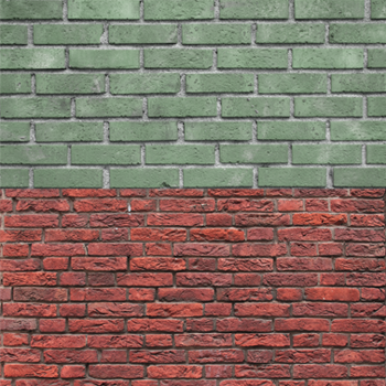
One way to deal with this problem is to pre-process the image, and leave only significant points, and apply subsequent algorithms to them. For this purpose, SIFT, SURF and other DAISY, feature descriptors were invented. With their help, you can stitch pictures, match objects and do a lot of useful things, however these descriptors have their drawbacks. In particular, it is expected that the points found will be in some sense truly special and unique, reproducible from image to image. You should not use SIFT to understand that both halves of this image are brick walls.
')
In addition, although these descriptors are called local, they still use a fairly large area of the image. This is not a good computational cost. Let's weaken this position a little. Perhaps we can characterize the image, considering even smaller structures?
Again, we want to get a way to describe the structure of the picture, which
So what is a local binary pattern? In short: this is a way for each pixel to describe in which direction the brightness decreases. Build it is a snap. Let's do this and do it.
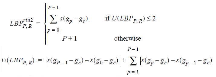
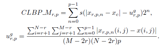
Wait a second, it's just a binary number! We will call it the buzzwords of Local Binary Pattern (Timo Ojala, July 2002). From the point of view of mathematics, it looks like this:
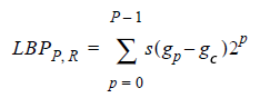
where s is a step (x) (step) function, which returns 0 if and 1 if . Are the brightness values of the pixel numbered neighbors, and - the brightness value of the center pixel itself.
That's all. A more savvy math reader would call the bits of the descriptor signs of brightness derivatives in directions, but this is unprincipled. It is clear that requirements 1-2 are trivially fulfilled. 3, probably, needs some work, we'll talk about it a little later. But what to do with 4? So far it is not entirely clear how to work with it. Yes, and with a decrease in the dimension of the problem, we coped so-so: instead of a byte of pixel brightness values, we got a byte of signs of brightness variation in directions. There are no invariance on affine transformations, but we didn’t demand it: after all, the pattern of squares and rhombuses are two different patterns.
From the obtained data it is already possible to extract something interesting, let's see how to put them into practice as soon as possible, and, proceeding from this, we will think about how to improve them.
Use LBP where you are working with textures. The most banal option: the program receives a texture at the input, and it determines the texture of what is in front of it. This may be one of the steps or an aid to a more complex algorithm. For example, the recognition algorithm in an image of an object that does not have a specific shape, but only some kind of structure: fire, smoke or foliage (Hongda Tian, 2011). Alternatively: use LBP when segmenting images to teach the machine to consider a unique object not every line on a zebra, but the whole zebra. See the trees behind the forest.
How exactly this happens depends on the task and the selected type of LBP. It does not always make sense to look at the pictures for repeating patterns from LBP, and certainly you should not compare descriptors on one image with descriptors on another. Resistance to noise, we plan to take quantity, and it plays with us a cruel joke: the resulting codes are simply too much. Good results can be obtained if the neural network autoencoder (autoencoder) is connected to the LBP card, it can extract more information from the prepared patterns than from the raw picture. A simpler option is to scrape all the resulting codes into one pile (build a histogram), and work with it already.
The latter approach looks strange at first. Is information not lost when we so simply erase information about the relative position of the trace elements in the image? In general, yes, it is possible to pick up an example from three pictures, that 1 and 2 are visually more similar, but according to the histogram, 1 and 3 are more similar, however, in practice this is unlikely.
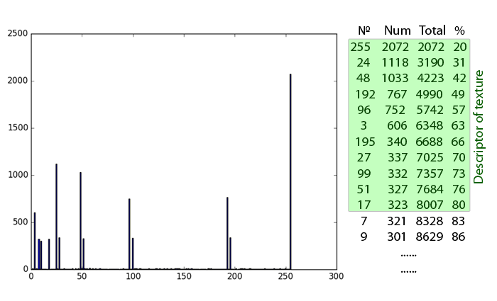
A full histogram also often carries redundant information, so I advise you to arm yourself with the technique proposed in (S. Liao, May 2009) and developed in (Jinwang Feng, 2015):
In conclusion, I note that no one forces you to dwell on textures. LBPs are successfully applied instead of and along with Haar-like features in AdaBoost training. They capture high-frequency information that integral features miss.
So far, the choice of LBP as low-level information for machine learning looks unconvincing. It's time to fix the flaws that we talked about above! For such a surprisingly simple descriptor as LBP during its existence, many variations have been invented.
We have two conflicting tasks. First: reduce the number of patterns to make it easier to chew on the machine. Often we are interested in histograms, and if a histogram of 2 ^ 8 elements is acceptable, then from 2 ^ 24 it takes up a lot of space. Second: to increase the information content of the patterns. We would like to distinguish particular points of different types, and, the more they differ, the more patterns should differ. A separate item should be made resistance to noise.
To begin with, we note that the objects that the human eye can recognize are the most interesting for us: the boundaries of lines, corners, points, or spots. If you mentally place the center point on the edge of such an object and calculate the LBP, then at the circle stage you can see that the zeros and ones are divided into two groups. When the circle is “drawn out”, a number with 0, 1 or 2 transitions 0-1 or 1-0 is formed. For example, "00111100", "11111111" and "01111111" - refer to the "good" patterns, and "10100000" and "01010101" - no.
Rejoice. Although not that we are the only ones who discovered it. In the work with which the active LBP study began (Timo Ojala, July 2002), they also noticed that such patterns carry most of the relevant information. They even came up with a special name: “uniform patterns” (uniform patterns). Their number is easy to calculate: for 8 neighbors, we have 1 + 2 + 3 + 4 + 5 + 6 + 7 + 8 + 1 = 37 pieces ((P + 1) * P / 2 + 1). Plus, another label, under which we scrape together all the non-uniform patterns. It has become much more pleasant.
There are other ways to thin a set of tags. For example, if for some reason we don’t want to remove non-uniform patterns, we can at least get rid of all the patterns that result from rotating the image around the central pixel. Just enter a one-to-one correspondence that will display the LBP group into one. Let's say we will consider the “real” pattern as the one that has the minimum value in cyclic shifts to the right. Or to the left. The gift gets the invariance of the descriptor relative to the rotation of the object. (Junding Sun, 2013)

You can also take the same patterns, for cases where the object and the background change colors. Then it can be considered as a “effective” minimum pattern from LBP and ~ LBP. This option was used in the work of detecting smoke, which may look light gray against a dark background or dark gray against a white background (Hongda Tian, 2011).
In (Yiu-ming Cheung, 2014), it is generally proposed to get rid of unnecessary neighbors and count ultra-local descriptors using only a couple of pixels, and then “collect” features by calculating the coincidence matrices (co-occurrence matrix), but this is more like the usual calculation of the derivative with subsequent frauds over it. It seems to me difficult to effectively put them into practice.
Alternatively, we can consider the derivative of the brightness of the second order, it needs only 4 directions. Unfortunately, it is more prone to the negative effects of noise, and is less likely to carry significant information about the image. The use of this technique also strongly depends on the task.
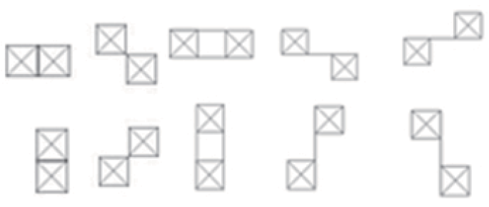
But in general, the idea of changing the way we consider a derivative was good. Let us try to return to the first derivative and introduce stricter restrictions on the change of its sign. We will consider not the directions from the central pixel to the outermost, but the directions from the outermost pixels to the outermost pixels from it (Junding Sun, 2013).
We will write a unit for a pixel if the brightness decreases from the first pixel to the central one and from the central one to the second. If the brightness increases or does not have a specific behavior - zero. Unfortunately, we lose information about bright and dark lonely points, but if we know that the image contains a lot of noise, it is even good.
In general, if a high level of noise is expected, more points can be used to calculate the derivative, averaged with some weights with the values of the neighbors or even pixel values outside the selected circle.
The way we check whether the brightness changes also seems a bit suspicious. In fact, if you just use the derivative symbol, then LBP will find phantom patterns even on an absolutely smooth image with even minimal noise. The usual way to deal with such a problem is to set a threshold with which we compare the change in brightness between pixels. You can set it from the outside if there is additional information about the character of the image, but this is not too great, since typical guessing on the parameters begins. The preferred option is to calculate the average value of the derivative over a certain neighborhood or the entire image and compare it with it (Jinwang Feng, 2015).
If you wish, you can use more gradations, but this inflates the maximum number of patterns.
Local Binary Pattern is easy to extend to the case of three dimensions (Xiaofeng Fu, 2012), (Guoying Zhao, 2007), (Xie Liping, July 2014). If you imagine the video as a “stack” of frames, then each pixel is not 8, but 9 + 9 + 8 = 26 neighbors (or less, if you remove some corner pixels). There are different ways to get LBP in this case. The two most common:
Finally, the result of some non-local filter can be attached to the descriptor. For example, in (Xie Liping, July 2014) Gabor filters are used for this. They are well suited for detecting periodic structures, but they have certain disadvantages, in particular, they “ring” on single direct lines. Proper combined use of LBP and global filters eliminates the drawbacks of both those and those. On Habré about the use of filters Gabor can be read, for example, here and here .
Practice without theory is blind, but theory without practice is completely dead, so let's program something already. This trivial Python 3.4 code (PIL, numpy and matplotlib required) counts and displays the LBP histogram for the image. For ease of understanding, only optimization was used with setting the minimum difference in brightness proportional to the average difference in brightness in the image. From the result, you can calculate and use DLBP for machine learning, but in general, this is a very naive implementation. In real-world applications, pre-processing is required. Note that zeros, descriptors of a homogeneous region are not recorded: they are almost always very, very much and they bring down the histogram normalization. They can be used separately as a measure of the scale of the texture.
Code:
Texture examples and results:
Notice that the same bins often have the highest values — they correspond to the uniform patterns discussed above. However, the distribution of them for different textures is different. The higher the noise level and randomness of the texture, the greater the “garbage” LBPs (see small bins in histograms).
Introduction
The LBP theme has already been raised on Habré, however, I decided to slightly spread the proposed explanation and share some variations of this pattern.
As you know, a computer image is the same numerical information. Each pixel is represented by a number in the case of a black and white image or a triple of numbers in the case of color. In general, they constitute a pleasant picture for the human eye and it is convenient to carry out transformations on them, but often there is too much information. For example, in object recognition tasks we rarely care about the value of each pixel separately: images are often noisy, and the desired images may appear in different versions, therefore it is desirable that the algorithms are resistant to errors, the ability to grasp the general trend. This property of English-speaking sources is called robustness.
One way to deal with this problem is to pre-process the image, and leave only significant points, and apply subsequent algorithms to them. For this purpose, SIFT, SURF and other DAISY, feature descriptors were invented. With their help, you can stitch pictures, match objects and do a lot of useful things, however these descriptors have their drawbacks. In particular, it is expected that the points found will be in some sense truly special and unique, reproducible from image to image. You should not use SIFT to understand that both halves of this image are brick walls.
')
In addition, although these descriptors are called local, they still use a fairly large area of the image. This is not a good computational cost. Let's weaken this position a little. Perhaps we can characterize the image, considering even smaller structures?
main idea
Again, we want to get a way to describe the structure of the picture, which
- Quickly considered
- Invariant under brightness conversions that preserve order (
 )
) - Noise resistant
- Resistant to texture variations
- Strongly reduces the dimension of the problem
So what is a local binary pattern? In short: this is a way for each pixel to describe in which direction the brightness decreases. Build it is a snap. Let's do this and do it.
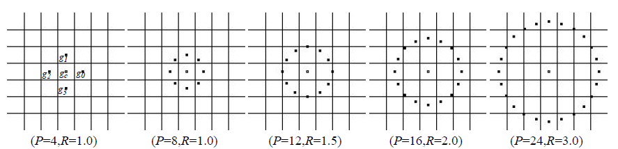
- First you need to choose the radius and the number of points ... stop-stop, who said "rogue"? Yes, literally a couple of lines above, I wrote that this descriptor is very local, but the definition of what is “very local” may differ from image to image. But so be it, let's stop at a radius of one: hereinafter, for each pixel, we will calculate LBP based on 8 adjacent points.
- Number the selected points.
- Calculate the difference in brightness values between each of the extreme pixels and the central one.
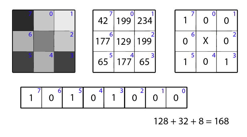
- If the difference is negative (brightness decreases), write one in the mind of the neighbor’s place, if nonnegative (> = 0) is zero.
- “Pull” the resulting circle from zeros and ones into a line.
Wait a second, it's just a binary number! We will call it the buzzwords of Local Binary Pattern (Timo Ojala, July 2002). From the point of view of mathematics, it looks like this:
where s is a step (x) (step) function, which returns 0 if and 1 if . Are the brightness values of the pixel numbered neighbors, and - the brightness value of the center pixel itself.
That's all. A more savvy math reader would call the bits of the descriptor signs of brightness derivatives in directions, but this is unprincipled. It is clear that requirements 1-2 are trivially fulfilled. 3, probably, needs some work, we'll talk about it a little later. But what to do with 4? So far it is not entirely clear how to work with it. Yes, and with a decrease in the dimension of the problem, we coped so-so: instead of a byte of pixel brightness values, we got a byte of signs of brightness variation in directions. There are no invariance on affine transformations, but we didn’t demand it: after all, the pattern of squares and rhombuses are two different patterns.
From the obtained data it is already possible to extract something interesting, let's see how to put them into practice as soon as possible, and, proceeding from this, we will think about how to improve them.
Well, I learned to count LBP. What's next?
Use LBP where you are working with textures. The most banal option: the program receives a texture at the input, and it determines the texture of what is in front of it. This may be one of the steps or an aid to a more complex algorithm. For example, the recognition algorithm in an image of an object that does not have a specific shape, but only some kind of structure: fire, smoke or foliage (Hongda Tian, 2011). Alternatively: use LBP when segmenting images to teach the machine to consider a unique object not every line on a zebra, but the whole zebra. See the trees behind the forest.
How exactly this happens depends on the task and the selected type of LBP. It does not always make sense to look at the pictures for repeating patterns from LBP, and certainly you should not compare descriptors on one image with descriptors on another. Resistance to noise, we plan to take quantity, and it plays with us a cruel joke: the resulting codes are simply too much. Good results can be obtained if the neural network autoencoder (autoencoder) is connected to the LBP card, it can extract more information from the prepared patterns than from the raw picture. A simpler option is to scrape all the resulting codes into one pile (build a histogram), and work with it already.
The latter approach looks strange at first. Is information not lost when we so simply erase information about the relative position of the trace elements in the image? In general, yes, it is possible to pick up an example from three pictures, that 1 and 2 are visually more similar, but according to the histogram, 1 and 3 are more similar, however, in practice this is unlikely.
A full histogram also often carries redundant information, so I advise you to arm yourself with the technique proposed in (S. Liao, May 2009) and developed in (Jinwang Feng, 2015):
- Calculate descriptors for each pixel in the image.
- Count their histogram
- Sort the histogram beans descending. Surprisingly, according to (S. Liao, May 2009), information about which bins can be discarded, their very distribution by the histogram carries enough information. You can not discard, in my opinion, so reliable.
- Leave the part of the histogram, which includes a certain predetermined percentage of patterns, discard the rest. Charts in the same paper claim that 80% is an acceptable number. The left part of the distribution ([bin number], its percentage) is the so-called dominant patterns (DLBP).
- DLBP can be fed to a neural network or SVM, which, with the help of machine learning magic and a previously provided training set, will determine what kind of texture is in front of it.
In conclusion, I note that no one forces you to dwell on textures. LBPs are successfully applied instead of and along with Haar-like features in AdaBoost training. They capture high-frequency information that integral features miss.
Variations
So far, the choice of LBP as low-level information for machine learning looks unconvincing. It's time to fix the flaws that we talked about above! For such a surprisingly simple descriptor as LBP during its existence, many variations have been invented.
We have two conflicting tasks. First: reduce the number of patterns to make it easier to chew on the machine. Often we are interested in histograms, and if a histogram of 2 ^ 8 elements is acceptable, then from 2 ^ 24 it takes up a lot of space. Second: to increase the information content of the patterns. We would like to distinguish particular points of different types, and, the more they differ, the more patterns should differ. A separate item should be made resistance to noise.
Significant patterns
To begin with, we note that the objects that the human eye can recognize are the most interesting for us: the boundaries of lines, corners, points, or spots. If you mentally place the center point on the edge of such an object and calculate the LBP, then at the circle stage you can see that the zeros and ones are divided into two groups. When the circle is “drawn out”, a number with 0, 1 or 2 transitions 0-1 or 1-0 is formed. For example, "00111100", "11111111" and "01111111" - refer to the "good" patterns, and "10100000" and "01010101" - no.
Rejoice. Although not that we are the only ones who discovered it. In the work with which the active LBP study began (Timo Ojala, July 2002), they also noticed that such patterns carry most of the relevant information. They even came up with a special name: “uniform patterns” (uniform patterns). Their number is easy to calculate: for 8 neighbors, we have 1 + 2 + 3 + 4 + 5 + 6 + 7 + 8 + 1 = 37 pieces ((P + 1) * P / 2 + 1). Plus, another label, under which we scrape together all the non-uniform patterns. It has become much more pleasant.
There are other ways to thin a set of tags. For example, if for some reason we don’t want to remove non-uniform patterns, we can at least get rid of all the patterns that result from rotating the image around the central pixel. Just enter a one-to-one correspondence that will display the LBP group into one. Let's say we will consider the “real” pattern as the one that has the minimum value in cyclic shifts to the right. Or to the left. The gift gets the invariance of the descriptor relative to the rotation of the object. (Junding Sun, 2013)
You can also take the same patterns, for cases where the object and the background change colors. Then it can be considered as a “effective” minimum pattern from LBP and ~ LBP. This option was used in the work of detecting smoke, which may look light gray against a dark background or dark gray against a white background (Hongda Tian, 2011).
In (Yiu-ming Cheung, 2014), it is generally proposed to get rid of unnecessary neighbors and count ultra-local descriptors using only a couple of pixels, and then “collect” features by calculating the coincidence matrices (co-occurrence matrix), but this is more like the usual calculation of the derivative with subsequent frauds over it. It seems to me difficult to effectively put them into practice.
Alternatively, we can consider the derivative of the brightness of the second order, it needs only 4 directions. Unfortunately, it is more prone to the negative effects of noise, and is less likely to carry significant information about the image. The use of this technique also strongly depends on the task.
Noise resistance
But in general, the idea of changing the way we consider a derivative was good. Let us try to return to the first derivative and introduce stricter restrictions on the change of its sign. We will consider not the directions from the central pixel to the outermost, but the directions from the outermost pixels to the outermost pixels from it (Junding Sun, 2013).
We will write a unit for a pixel if the brightness decreases from the first pixel to the central one and from the central one to the second. If the brightness increases or does not have a specific behavior - zero. Unfortunately, we lose information about bright and dark lonely points, but if we know that the image contains a lot of noise, it is even good.
In general, if a high level of noise is expected, more points can be used to calculate the derivative, averaged with some weights with the values of the neighbors or even pixel values outside the selected circle.
The way we check whether the brightness changes also seems a bit suspicious. In fact, if you just use the derivative symbol, then LBP will find phantom patterns even on an absolutely smooth image with even minimal noise. The usual way to deal with such a problem is to set a threshold with which we compare the change in brightness between pixels. You can set it from the outside if there is additional information about the character of the image, but this is not too great, since typical guessing on the parameters begins. The preferred option is to calculate the average value of the derivative over a certain neighborhood or the entire image and compare it with it (Jinwang Feng, 2015).
If you wish, you can use more gradations, but this inflates the maximum number of patterns.
More information
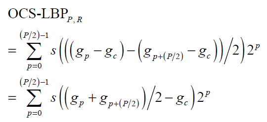
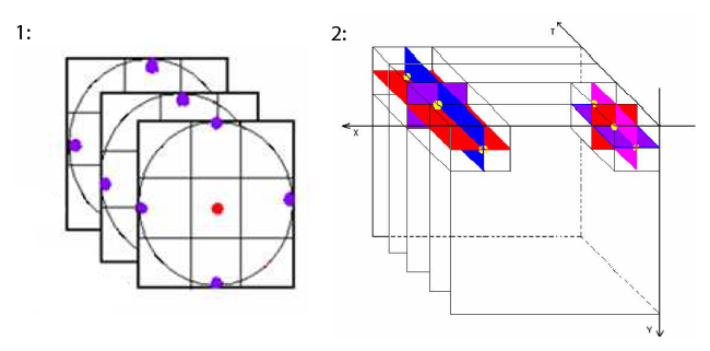
Local Binary Pattern is easy to extend to the case of three dimensions (Xiaofeng Fu, 2012), (Guoying Zhao, 2007), (Xie Liping, July 2014). If you imagine the video as a “stack” of frames, then each pixel is not 8, but 9 + 9 + 8 = 26 neighbors (or less, if you remove some corner pixels). There are different ways to get LBP in this case. The two most common:
- Three parallel to the plane. For each pixel i, j, we calculate by the standard LBP in frames t-1, t, t + 1. Then we concatenate them and write them down, or, if we are only interested in patterns that do not change from frame to frame, we compare them to each other, and we write only if the resulting LBPs are the same, otherwise we assign a garbage tag.
- Three orthogonal planes. For each pixel (i, j, t), we consider three sets of neighbors: those lying in the frame, different in time, the same in a row, different in time and the same in a column. This method is more suitable for patterns that change over time. It requires more computational expense than the previous one.
Finally, the result of some non-local filter can be attached to the descriptor. For example, in (Xie Liping, July 2014) Gabor filters are used for this. They are well suited for detecting periodic structures, but they have certain disadvantages, in particular, they “ring” on single direct lines. Proper combined use of LBP and global filters eliminates the drawbacks of both those and those. On Habré about the use of filters Gabor can be read, for example, here and here .
Example
Practice without theory is blind, but theory without practice is completely dead, so let's program something already. This trivial Python 3.4 code (PIL, numpy and matplotlib required) counts and displays the LBP histogram for the image. For ease of understanding, only optimization was used with setting the minimum difference in brightness proportional to the average difference in brightness in the image. From the result, you can calculate and use DLBP for machine learning, but in general, this is a very naive implementation. In real-world applications, pre-processing is required. Note that zeros, descriptors of a homogeneous region are not recorded: they are almost always very, very much and they bring down the histogram normalization. They can be used separately as a measure of the scale of the texture.
Code:
(I beg your pardon for deviating from style in the name of simplicity)
from PIL import Image import matplotlib.pyplot as plt import numpy as np def compute_direction(x, y, threshold_delta): return 1 if x - y > threshold_delta else 0 # 7 0 1 # 6 x 2 # 5 4 3 def compute_lbp(data, i, j, threshold_delta): result = 0 result += compute_direction(data[i, j], data[i-1, j], threshold_delta) result += 2 * compute_direction(data[i, j], data[i-1, j+1], threshold_delta) result += 4 * compute_direction(data[i, j], data[i, j+1], threshold_delta) result += 8 * compute_direction(data[i, j], data[i+1, j+1], threshold_delta) result += 16 * compute_direction(data[i, j], data[i+1, j], threshold_delta) result += 32 * compute_direction(data[i, j], data[i+1, j-1], threshold_delta) result += 64 * compute_direction(data[i, j], data[i, j-1], threshold_delta) result += 128 * compute_direction(data[i, j], data[i-1, j-1], threshold_delta) return result image = Image.open("test.png", "r") image = image.convert('L') #makes it grayscale data = np.asarray(image.getdata(), dtype=np.float64).reshape((image.size[1], image.size[0])) lbps_histdata = [] mean_delta = 0 for i in range(1, image.size[1]-1): for j in range(1, image.size[0]-1): mean_delta += (abs(data[i, j] - data[i, j-1]) + abs(data[i, j] - data[i-1, j-1]) + abs(data[i, j] - data[i-1, j]) + abs(data[i, j] - data[i-1, j+1]) )/4.0 mean_delta /= (image.size[1]-2) * (image.size[0]-2) #normalizing mean_delta *= 1.5 #we are interested in distinct luminosity changes so let's rise up threshold for i in range(0, image.size[1]): for j in range(0, image.size[0]): if i != 0 and j != 0 and i != image.size[1]-1 and j != image.size[0]-1: tmp = compute_lbp(data, i, j, mean_delta) if tmp != 0: lbps_histdata.append(tmp) hist, bins = np.histogram(lbps_histdata, bins=254, normed=True) width = bins[1] - bins[0] center = (bins[:-1] + bins[1:]) / 2 plt.bar(center, hist, align='center', width=width) plt.show() Texture examples and results:
More pixels
And you call this textures? Well this is just patterns!
Well…

Pictures are specially selected so that the eye can see the similarities / differences. It is also easy to see why there are many / few LBPs in a particular pattern.
Pattern 1

Pattern 1 + noise

Pattern 1 + even more noise and spots

Pattern 2

Pattern 3

Well…
Pictures are specially selected so that the eye can see the similarities / differences. It is also easy to see why there are many / few LBPs in a particular pattern.
Pattern 1
Pattern 1 + noise
Pattern 1 + even more noise and spots
Pattern 2
Pattern 3
More pixels
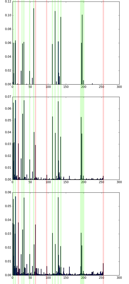
Comparison of LBP histograms of the first three pictures. The most characteristic bins coincide, but there are several parasitic ones. Note a large number of LBP = 255, black dots on a white background. Green coincidence marked, red - extra bins.
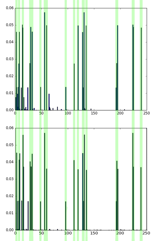
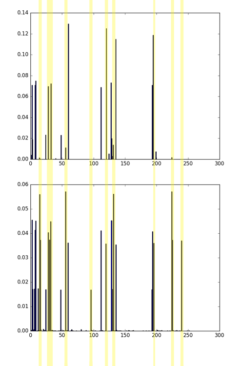
Comparison of histograms 4 and 5 pictures, then comparison of histograms 1 and 4 pictures. Greens are coincidences, yellow - differences. Although these pictures have different textures, 4 and 5 are definitely more similar than 1 and 4. This can be seen both by eye and by comparing histograms.
Comparison of histograms 4 and 5 pictures, then comparison of histograms 1 and 4 pictures. Greens are coincidences, yellow - differences. Although these pictures have different textures, 4 and 5 are definitely more similar than 1 and 4. This can be seen both by eye and by comparing histograms.
Notice that the same bins often have the highest values — they correspond to the uniform patterns discussed above. However, the distribution of them for different textures is different. The higher the noise level and randomness of the texture, the greater the “garbage” LBPs (see small bins in histograms).
List of sources
- Dong-Chen He, LN (1989). Texture Unit, Texture Spectrum, And Texture Analysis. Geoscience and Remote Sensing Symposium.
- Guoying Zhao, MP (2007). Dynamic Texture Recognition Using Facial Expressions. IEEE Transactions on Pattern Analysis and Machine Intelligence.
- Hongda Tian, WL (2011). Smoke Detection Using Non-Redundant Local Binary Pattern-Based Features. Wollongong, Australia: Advanced Multimedia Research Lab, ICT Research Institute.
- Jinwang Feng, YD (2015). Dominant – Completed Local Binary Pattern for Texture Classification. Materials of International Conference on Information and Automation. Lijiang, China.
- Junding Sun, GF (2013). New Local Edge Binary Patterns For Image Retrieval.
- S. Liao, MW (May 2009). Dominant Local Binary Patterns for Texture Classification. Transactions on Image Processing, Vol 18, No 5.
- T. Ojala, MP (1994). Discrimination based on Kullback discrimination of distributions. Vol. 1 - Proceedings of the 12th IAPR International Conference on Computer Vision & Image Processing.
- Timo Ojala, MP (July 2002). Gray Scale and Rotation Invariant Texture Classification. IEEE Transactions on Pattern Analysis and Machine Intelligence, 971-987.
- Xiaofeng Fu, RW (2012). Spatiotemporal Pattern Orientational Binary Patterns for Facial Expression Recognition from Video Sequences. International Conference on Fuzzy Systems and Knowledge Discovery.
- Xie Liping, WH (July 2014). Facial Expression Recognition Using Histogram Sequence of Biblical Patterns from Three Orthogonal Planes. Proceedings of the 33rd Chinese Control Conference. Nanjing, China.
- Yiu-ming Cheung, JD (2014). Ultra Local Binary Pattern For Image Texture Analysis. Materials of IEEE International Conference on Security, Pattern Analysis, and Cybernetics. Wuhan, Hibei, China.
Source: https://habr.com/ru/post/280888/
All Articles