FlashSort sorting method
Hello to all!
I have one hobby - I really like reinventing bicycles.
About the invention of one such bike I want to tell you today.
Sorting an array of data is a task that is far from being the first year. She pursues us from the first courses of technical universities, and who are particularly lucky, and from school. These are usually methods of sorting by “bubble”, “division”, “fast”, “inserts” and others.
')

Here, for example, a similar implementation of the bubble sorting method was taught to me in a large IT company. This method has been used by experienced programmers everywhere.
So, I was always wondering why so little attention is paid to sorting methods without comparison (bitwise, block, etc.). After all, such methods belong to the class of fast algorithms, are performed in O (N) the number of reads and permutations and, with well-chosen data, can be performed in linear time. Of course, they are poorly suited for sorting some abstract objects, since these methods, in fact, do not compare anything, but take some kind of digit from the value (although with a special desire, you can add and sort objects). However, in practice, most sorting tasks are reduced to ordering an array of ordinary primitives: strings, numbers, bit fields, etc., where the comparison is mostly byte-by-byte.
If, for example, we are talking about the pocket sorting method, then Wikipedia claims that it does not work well with a large number of little-different elements or the unsuccessful function of getting the basket number from the contents of the element. The algorithm requires knowing the nature of the data being sorted. Additionally, you need to organize pockets, which eats away processor time and memory. However, despite all the flaws, potentially, the execution time of the algorithm in theory tends to be linear. Is it possible to somehow solve these shortcomings and achieve a linear execution time?
So, I offer you a sorting algorithm with O (N) number of reads and permutations and with the execution time “close” to linear.
The algorithm sorts the source data in-place and does not use additional memory. In other words, sorting with O (N) number of readings, displacements and memory O (1).
The sorting method is based on the pocket sorting method. If we talk about a specific implementation, for a more efficient comparison of elements byte by byte the number of pockets is chosen equal to 256. The number of iterations (passes) depends on the length of one element in bytes. Those. the total number of permutations will be O (N * K), where K is the length (number of bytes) of one element.
To sort, we need to use a special buffer - “pockets”. This is an array of length 256, each element of which contains the size of the pocket and a link to the border of the pocket — this is a pointer to the first element of the pocket in the source array. Initially, the buffer is initialized with zeros.
So, the sorting algorithm for each i-th iteration consists of four stages.
Stage 1. Counting Pocket Size
At the first stage, pocket sizes are calculated. We use our buffer, where for each pocket will be counted the number of items. We go over all elements, take the value of the i-th byte and increment the counter for the corresponding pocket.
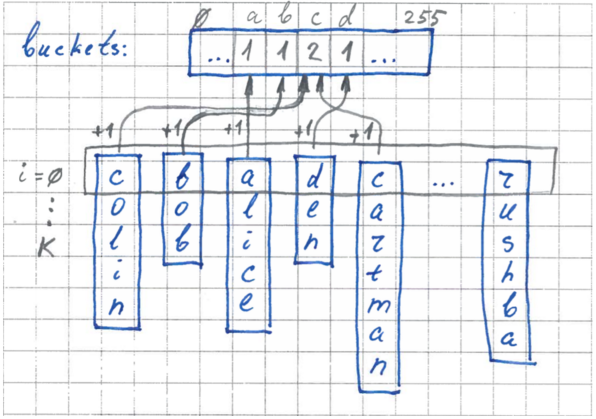
Stage 2 Setting borders
Now, knowing the dimensions of each pocket, we can clearly set the boundaries in our original array for each pocket. We run over our buffer and set the boundaries - set pointers to the elements for each pocket.

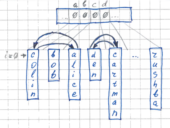
Stage 3 Permutation
In the second pass, we rearrange the elements in the original array so that each of them is in its place, in its pocket.
The permutation algorithm is as follows:
During each permutation, the counters in the buffer for the corresponding pocket will be decremented back, and by the end of the run our buffer will be filled with zeros again and ready for use at other iterations.
The permutation process, like the first stage, will theoretically be carried out in linear time, since the number of permutations will never exceed N — the number of elements.
4 stage. Recursive descent
And the last stage. Now we recursively sort the elements inside each formed pocket. For each inner iteration, you only need to know the border of the current pocket. Since we do not use additional memory (information about the length of the current pocket has not been preserved anywhere), before going to the inner iteration, we run over the elements again and calculate the length of the current pocket.

If desired, this can be avoided by further optimizing the algorithm and not deleting information about pocket lengths. However, this will require additional memory. In particular, O (log (K) * M), where M is the number of pockets (in our case it is always 256), K is the length of one element (in bytes).
A distinctive feature of the algorithm is that during the first pass (step No. 1), the number of the first and last non-empty pocket is additionally remembered (pointers pBucketLow, pBucketHigh). In the future, this will save time at the 2nd and 3rd stages. This optimization assumes that most of the data is concentrated in a certain range of data and often has some defined boundaries. For example, string data often begins with the character AZ. Numbers (such as ID) are also usually limited to a range.
Additional optimization can also be carried out if the numbers of the lower and upper non-empty pockets match (pBucketLow == pBucketHigh). This suggests that all elements at the i-th level have the same byte, and all elements fall into one pocket. In this case, we can immediately interrupt the iteration (skip 2,3,4 stages) and move on to the next one.
The algorithm also uses another fairly common optimization. Before starting any iteration, in the case when the number of elements is small (in particular, less than 8), it is better to perform some very simple sorting (for example, bubble-sort).
The implementation of the above C algorithm is available on github: github.com/denisskin/cflashsort
To sort the data, you need to use the flash_sort function, which takes a pointer to the get_byte (void *, int) function as a parameter - the function to get the i-th element byte.
For example, sort the lines:
There is also a flashsort_const function for sorting data of a strictly specified length.
For example, numbers:
This function can also be successfully used to sort an array of structures by key.
For example:
For obvious reasons, the flashsort_const function will work a little slower than its counterpart - a function that was declared using a special macro. In this case, the permutation of elements and the receipt of the i-th byte of the element will occur much faster.
For example, you can declare the function of sorting numbers using a macro as follows:
In the same repository, you can also find benchmarks, where for comparison, sorting with the qsort method is added.
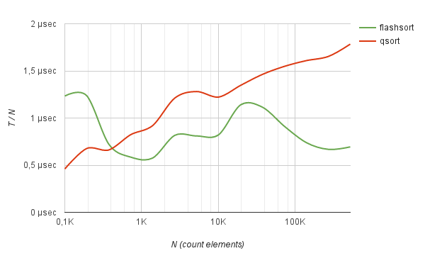
As a result, the flash_sort method shows itself well in comparison with qsort in working with randomly distributed data. For example, sorting an array of 500K int numbers works 2.5 times faster than quick-sort. As can be seen from the benchmark, the average sorting time divided by N, with an increase in the number of elements, does not practically change.
Benchmarks sorting of integers
Similar results are produced by sorting random strings of a given length. For example, a list of random hashes encoded in base64.
benchmark Sorting of hashes base64
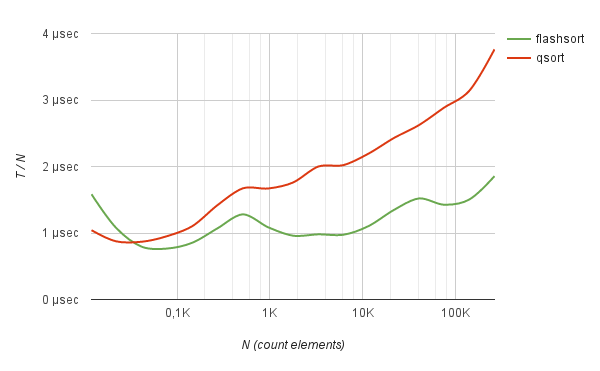
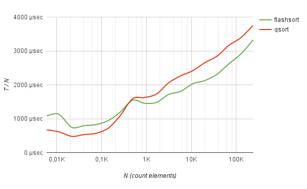
However, the method works without a clear advantage: only slightly faster than quick-sort while sorting randomly mixed English words.
benchmark Sorting of english words
Not bad the method shows itself in work with often-repeating data. For example, sorting logs of half a million IP addresses (taken from real life) using the flash-sort method works 5 times faster than quick sorting.
benchmark Sorting of IP addresses log
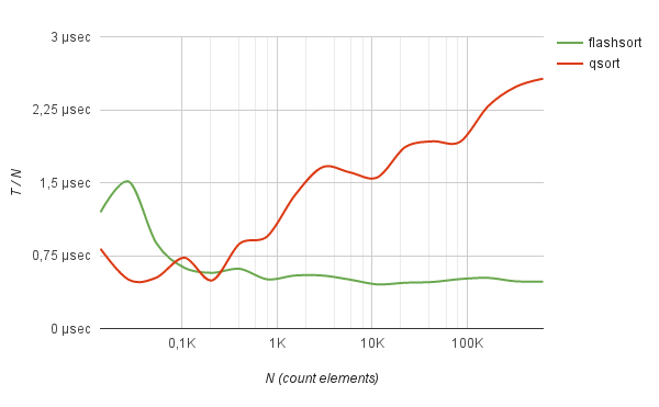
Moreover, on such data, the sorting time grows strictly linearly with the number of elements being sorted.
Although the sorting method presented here always does strictly O (N) reads and permutations, it would still be naive to expect that for all data types in all cases the algorithm will work in linear time. It is quite obvious that in practice its speed will depend on the nature of the data being sorted.
The execution of the algorithm in the general case will occur in nonlinear time, if only because at the stage of rearranging elements it needs to access random parts of the memory.
However, I believe that there is still room for optimization of the method described here. For example, at the first stage of the algorithm, in addition to counting the number of elements falling into the basket, it is possible to keep some more complex statistics and, on its basis, to choose various methods for sorting the elements inside the basket. I am sure that ultimately a good solution could be the development of such a hybrid algorithm that combines the approaches of various sorting methods, as well as optimization for a specific physical representation of data in memory or on disk.
However, these questions are beyond the scope of the article, the purpose of which was only to show the possibilities of the sorting methods “not by comparison” in their pure form. In any case, I think that it is still too early to put an end to data sorting issues.
I have one hobby - I really like reinventing bicycles.
About the invention of one such bike I want to tell you today.
Sorting an array of data is a task that is far from being the first year. She pursues us from the first courses of technical universities, and who are particularly lucky, and from school. These are usually methods of sorting by “bubble”, “division”, “fast”, “inserts” and others.
')
Here, for example, a similar implementation of the bubble sorting method was taught to me in a large IT company. This method has been used by experienced programmers everywhere.
So, I was always wondering why so little attention is paid to sorting methods without comparison (bitwise, block, etc.). After all, such methods belong to the class of fast algorithms, are performed in O (N) the number of reads and permutations and, with well-chosen data, can be performed in linear time. Of course, they are poorly suited for sorting some abstract objects, since these methods, in fact, do not compare anything, but take some kind of digit from the value (although with a special desire, you can add and sort objects). However, in practice, most sorting tasks are reduced to ordering an array of ordinary primitives: strings, numbers, bit fields, etc., where the comparison is mostly byte-by-byte.
If, for example, we are talking about the pocket sorting method, then Wikipedia claims that it does not work well with a large number of little-different elements or the unsuccessful function of getting the basket number from the contents of the element. The algorithm requires knowing the nature of the data being sorted. Additionally, you need to organize pockets, which eats away processor time and memory. However, despite all the flaws, potentially, the execution time of the algorithm in theory tends to be linear. Is it possible to somehow solve these shortcomings and achieve a linear execution time?
So, I offer you a sorting algorithm with O (N) number of reads and permutations and with the execution time “close” to linear.
The algorithm sorts the source data in-place and does not use additional memory. In other words, sorting with O (N) number of readings, displacements and memory O (1).
The sorting method is based on the pocket sorting method. If we talk about a specific implementation, for a more efficient comparison of elements byte by byte the number of pockets is chosen equal to 256. The number of iterations (passes) depends on the length of one element in bytes. Those. the total number of permutations will be O (N * K), where K is the length (number of bytes) of one element.
To sort, we need to use a special buffer - “pockets”. This is an array of length 256, each element of which contains the size of the pocket and a link to the border of the pocket — this is a pointer to the first element of the pocket in the source array. Initially, the buffer is initialized with zeros.
So, the sorting algorithm for each i-th iteration consists of four stages.
Stage 1. Counting Pocket Size
At the first stage, pocket sizes are calculated. We use our buffer, where for each pocket will be counted the number of items. We go over all elements, take the value of the i-th byte and increment the counter for the corresponding pocket.
Stage 2 Setting borders
Now, knowing the dimensions of each pocket, we can clearly set the boundaries in our original array for each pocket. We run over our buffer and set the boundaries - set pointers to the elements for each pocket.
Stage 3 Permutation
In the second pass, we rearrange the elements in the original array so that each of them is in its place, in its pocket.
The permutation algorithm is as follows:
- Run in order for all elements of the array. For the current element we take its i-th byte.
- If the current item is in its place (in its pocket), then everything is OK - move on to the next item.
- If the element is not in its place - the corresponding pocket is further, then we make a permutation with the element that is in this far pocket. Repeat this procedure until we get a suitable item with the right pocket. Each time we make a replacement, we put the current item in our pocket and do not re-analyze it again. Thus, the number of permutations will never exceed N.
During each permutation, the counters in the buffer for the corresponding pocket will be decremented back, and by the end of the run our buffer will be filled with zeros again and ready for use at other iterations.
The permutation process, like the first stage, will theoretically be carried out in linear time, since the number of permutations will never exceed N — the number of elements.
4 stage. Recursive descent
And the last stage. Now we recursively sort the elements inside each formed pocket. For each inner iteration, you only need to know the border of the current pocket. Since we do not use additional memory (information about the length of the current pocket has not been preserved anywhere), before going to the inner iteration, we run over the elements again and calculate the length of the current pocket.
If desired, this can be avoided by further optimizing the algorithm and not deleting information about pocket lengths. However, this will require additional memory. In particular, O (log (K) * M), where M is the number of pockets (in our case it is always 256), K is the length of one element (in bytes).
A distinctive feature of the algorithm is that during the first pass (step No. 1), the number of the first and last non-empty pocket is additionally remembered (pointers pBucketLow, pBucketHigh). In the future, this will save time at the 2nd and 3rd stages. This optimization assumes that most of the data is concentrated in a certain range of data and often has some defined boundaries. For example, string data often begins with the character AZ. Numbers (such as ID) are also usually limited to a range.
Additional optimization can also be carried out if the numbers of the lower and upper non-empty pockets match (pBucketLow == pBucketHigh). This suggests that all elements at the i-th level have the same byte, and all elements fall into one pocket. In this case, we can immediately interrupt the iteration (skip 2,3,4 stages) and move on to the next one.
The algorithm also uses another fairly common optimization. Before starting any iteration, in the case when the number of elements is small (in particular, less than 8), it is better to perform some very simple sorting (for example, bubble-sort).
Implementation
The implementation of the above C algorithm is available on github: github.com/denisskin/cflashsort
To sort the data, you need to use the flash_sort function, which takes a pointer to the get_byte (void *, int) function as a parameter - the function to get the i-th element byte.
For example, sort the lines:
// sort array of strings char *names[10] = { "Hunter", "Isaac", "Christopher", "Bob", "Faith", "Alice", "Gabriel", "Denis", "****", "Ethan", }; static const char* get_char(const void *value, unsigned pos) { return *((char*)value + pos)? (char*)value + pos : NULL; } flashsort((void**)names, 10, get_char); There is also a flashsort_const function for sorting data of a strictly specified length.
For example, numbers:
// sort integer values int nums[10] = {9, 6, 7, 0, 3, 1, 3, 2, 5, 8}; flashsort_const(nums, 10, sizeof(int), sizeof(int)); This function can also be successfully used to sort an array of structures by key.
For example:
// sort key-value array by key typedef struct { int key; char *value; } KeyValue; KeyValue names[10] = { {8, "Hunter"}, {9, "Isaac"}, {3, "Christopher"}, {2, "Bob"}, {6, "Faith"}, {1, "Alice"}, {7, "Gabriel"}, {4, "Denis"}, {0, "none"}, {5, "Ethan"}, }; flashsort_const(names, 10, sizeof(KeyValue), sizeof(names->key)); For obvious reasons, the flashsort_const function will work a little slower than its counterpart - a function that was declared using a special macro. In this case, the permutation of elements and the receipt of the i-th byte of the element will occur much faster.
For example, you can declare the function of sorting numbers using a macro as follows:
// define function flashsort_int by macro #define FLASH_SORT_NAME flashsort_int #define FLASH_SORT_TYPE int #include "src/flashsort_macro.h" int A[10] = {9, 6, 7, 0, 3, 1, 3, 2, 5, 8}; flashsort_int(A, 10); Benchmarks
In the same repository, you can also find benchmarks, where for comparison, sorting with the qsort method is added.
cd benchmarks gcc ../src/*.c benchmarks.c -o benchmarks.o && ./benchmarks.o As a result, the flash_sort method shows itself well in comparison with qsort in working with randomly distributed data. For example, sorting an array of 500K int numbers works 2.5 times faster than quick-sort. As can be seen from the benchmark, the average sorting time divided by N, with an increase in the number of elements, does not practically change.
Benchmarks sorting of integers
------------------------------------------------------------------------------------------- Count Flash-sort | Quick-sort | elements Total time | Total time | N Tf Tf / N | Tq Tq / N | Δ ------------------------------------------------------------------------------------------- 100 0.000012 sec 1.225 µs | 0.000004 sec 0.428 µs | -65.10 % 194 0.000016 sec 0.814 µs | 0.000009 sec 0.439 µs | -46.04 % 374 0.000026 sec 0.690 µs | 0.000023 sec 0.604 µs | -12.40 % 724 0.000043 sec 0.592 µs | 0.000058 sec 0.795 µs | +34.29 % 1398 0.000099 sec 0.707 µs | 0.000155 sec 1.112 µs | +57.28 % 2702 0.000204 sec 0.753 µs | 0.000300 sec 1.111 µs | +47.44 % 5220 0.000410 sec 0.786 µs | 0.000620 sec 1.187 µs | +51.02 % 10085 0.000845 sec 0.838 µs | 0.001254 sec 1.243 µs | +48.41 % 19483 0.002205 sec 1.132 µs | 0.002672 sec 1.372 µs | +21.21 % 37640 0.004242 sec 1.127 µs | 0.005436 sec 1.444 µs | +28.15 % 72716 0.006886 sec 0.947 µs | 0.011171 sec 1.536 µs | +62.23 % 140479 0.011156 sec 0.794 µs | 0.022899 sec 1.630 µs | +105.26% 271388 0.018773 sec 0.692 µs | 0.045749 sec 1.686 µs | +143.70% 524288 0.037429 sec 0.714 µs | 0.093858 sec 1.790 µs | +150.76% Similar results are produced by sorting random strings of a given length. For example, a list of random hashes encoded in base64.
benchmark Sorting of hashes base64
--------------------------------------------------------------------------------------------- Count Flash-sort | Quick-sort | elements Total time | Total time | N Tf Tf / N | Tq Tq / N | Δ --------------------------------------------------------------------------------------------- 147 0.000009 sec 0.609 µs | 0.000010 sec 0.694 µs | +13.97 % 274 0.000025 sec 0.918 µs | 0.000027 sec 0.991 µs | +7.95 % 512 0.000053 sec 1.036 µs | 0.000061 sec 1.195 µs | +15.37 % 955 0.000098 sec 1.024 µs | 0.000135 sec 1.416 µs | +38.32 % 1782 0.000164 sec 0.921 µs | 0.000279 sec 1.566 µs | +70.04 % 3326 0.000315 sec 0.947 µs | 0.000581 sec 1.745 µs | +84.31 % 6208 0.000629 sec 1.013 µs | 0.001210 sec 1.949 µs | +92.39 % 11585 0.001325 sec 1.144 µs | 0.002378 sec 2.053 µs | +79.50 % 21618 0.002904 sec 1.343 µs | 0.004712 sec 2.180 µs | +62.26 % 40342 0.006132 sec 1.520 µs | 0.009752 sec 2.417 µs | +59.03 % 75281 0.010780 sec 1.432 µs | 0.019778 sec 2.627 µs | +83.47 % 140479 0.023484 sec 1.672 µs | 0.043534 sec 3.099 µs | +85.37 % 262144 0.044967 sec 1.715 µs | 0.082878 sec 3.162 µs | +84.31 % However, the method works without a clear advantage: only slightly faster than quick-sort while sorting randomly mixed English words.
benchmark Sorting of english words
--------------------------------------------------------------------------------------------- Count Flash-sort | Quick-sort | elements Total time | Total time | N Tf Tf / N | Tq Tq / N | Δ --------------------------------------------------------------------------------------------- 140 0.000016 sec 1.166 µs | 0.000014 sec 0.993 µs | -14.85 % 261 0.000030 sec 1.168 µs | 0.000029 sec 1.114 µs | -4.59 % 485 0.000055 sec 1.139 µs | 0.000061 sec 1.259 µs | +10.59 % 901 0.000141 sec 1.565 µs | 0.000158 sec 1.750 µs | +11.82 % 1673 0.000269 sec 1.608 µs | 0.000315 sec 1.884 µs | +17.17 % 3106 0.000536 sec 1.726 µs | 0.000655 sec 2.110 µs | +22.27 % 5766 0.001013 sec 1.756 µs | 0.001263 sec 2.191 µs | +24.76 % 10703 0.002007 sec 1.875 µs | 0.002525 sec 2.359 µs | +25.85 % 19868 0.004152 sec 2.090 µs | 0.005150 sec 2.592 µs | +24.04 % 36880 0.008459 sec 2.294 µs | 0.010266 sec 2.784 µs | +21.36 % 68458 0.017460 sec 2.550 µs | 0.021423 sec 3.129 µs | +22.70 % 127076 0.035615 sec 2.803 µs | 0.041683 sec 3.280 µs | +17.04 % 235885 0.075747 sec 3.211 µs | 0.086523 sec 3.668 µs | +14.23 % Not bad the method shows itself in work with often-repeating data. For example, sorting logs of half a million IP addresses (taken from real life) using the flash-sort method works 5 times faster than quick sorting.
benchmark Sorting of IP addresses log
--------------------------------------------------------------------------------------------- Count Flash-sort | Quick-sort | elements Total time | Total time | N Tf Tf / N | Tq Tq / N | Δ --------------------------------------------------------------------------------------------- 107 0.000010 sec 0.953 µs | 0.000011 sec 1.056 µs | +10.78 % 208 0.000013 sec 0.639 µs | 0.000010 sec 0.480 µs | -25.00 % 407 0.000024 sec 0.584 µs | 0.000033 sec 0.812 µs | +39.01 % 793 0.000039 sec 0.493 µs | 0.000073 sec 0.915 µs | +85.61 % 1547 0.000080 sec 0.517 µs | 0.000211 sec 1.367 µs | +164.15% 3016 0.000169 sec 0.560 µs | 0.000512 sec 1.697 µs | +202.80% 5881 0.000308 sec 0.523 µs | 0.000962 sec 1.636 µs | +212.67% 11466 0.000548 sec 0.478 µs | 0.001812 sec 1.581 µs | +230.48% 22354 0.001034 sec 0.463 µs | 0.004191 sec 1.875 µs | +305.26% 43584 0.002109 sec 0.484 µs | 0.008693 sec 1.994 µs | +312.26% 84974 0.004411 sec 0.519 µs | 0.016003 sec 1.883 µs | +262.81% 165670 0.008837 sec 0.533 µs | 0.037358 sec 2.255 µs | +322.75% 323000 0.016046 sec 0.497 µs | 0.081251 sec 2.516 µs | +406.36% 629739 0.030895 sec 0.491 µs | 0.164283 sec 2.609 µs | +431.75% Moreover, on such data, the sorting time grows strictly linearly with the number of elements being sorted.
Finally
Although the sorting method presented here always does strictly O (N) reads and permutations, it would still be naive to expect that for all data types in all cases the algorithm will work in linear time. It is quite obvious that in practice its speed will depend on the nature of the data being sorted.
The execution of the algorithm in the general case will occur in nonlinear time, if only because at the stage of rearranging elements it needs to access random parts of the memory.
However, I believe that there is still room for optimization of the method described here. For example, at the first stage of the algorithm, in addition to counting the number of elements falling into the basket, it is possible to keep some more complex statistics and, on its basis, to choose various methods for sorting the elements inside the basket. I am sure that ultimately a good solution could be the development of such a hybrid algorithm that combines the approaches of various sorting methods, as well as optimization for a specific physical representation of data in memory or on disk.
However, these questions are beyond the scope of the article, the purpose of which was only to show the possibilities of the sorting methods “not by comparison” in their pure form. In any case, I think that it is still too early to put an end to data sorting issues.
Source: https://habr.com/ru/post/280848/
All Articles