Bayesian neural network is now orange (part 2)

What do you think, what's more in the orange - peel, or, hm, orange?



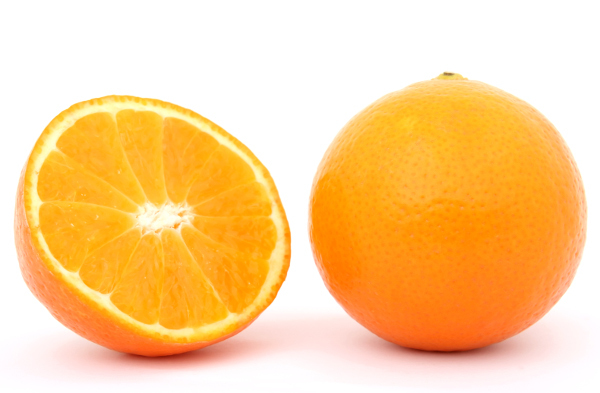
I suggest, if possible, go to the kitchen, take an orange, peel and check. If laziness or not at hand - let's use boring mathematics: we remember the volume of the ball from school. Let, say, the thickness of the peel is from radius then , ; subtract one from the other, divide the volume of the peel by the volume of the orange ... it turns out that the peel is about 16%. Not so little, by the way.
')
How about an orange in millennial space?

Going to the kitchen this time will fail; I suspect that not everyone knows the formula by heart, but Wikipedia helps us. We repeat similar calculations, and with interest we find that:

• firstly, in the thousand-dimensional hyperapellin the rind is larger than the pulp
• and secondly, it is about 246993291800602563115535632700000000000000 more than

That is, no matter how strange and controversial this may seem, but almost the entire volume of hyperepel'sin is contained in a negligibly thin layer just below its surface.

Let's start with this, perhaps.

Synopsis

This is the second part of the post , where before that we stopped at the fact that we found the main Grail - the a posteriori probability of the model parameters. Here it is, just in case: . Remember again that - these are the model parameters (neural network weights, for example), and - data from dataset (I slightly changed the notation, earlier instead of was , but we will need theta later).

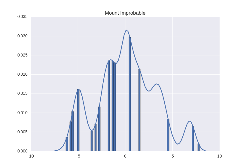
So, the orange is just that. The dimensions of this posterior grow with the same alarming speed, as the volume of hyperepel'sin; the more parameters we have, the “bigger” the distribution becomes. In fact, it is probably better to imagine not even an orange - let's imagine a mountain. In the millennial dimension. Yes, I know that it is slightly inconsistent, but the enive is a mountain:


This is all one-dimensional, true. According to the precepts of Hinton , you can imagine a thousand-meter mountain like this: look at the picture above and say “one thousand!” Loudly - or how many will be needed there.

Our challenge is to find out the volume of this mountain. However, we:
- we do not know what form it is (maybe any)
- (so far) we have only one method of measurement - standing at a point, we can calculate the height to the foot (the probability of being at this point)
- the surface of the mountain grows exponentially when it grows - similar to how the skin of hyperepelin grows

What is the plan?

Plan One: Sampling

We, generally speaking, do not need to measure the mountain right at every point. We can choose several random parts of the mountain, take measurements and outline the result. It will not be as accurate, but we will have to do much less measurements.
It can be noticed quite quickly that this idea is promising, but it will not help us much when our multidimensional mountain begins to grow with an increase in the number of dimensions. Let us recall that the surface of a mountain is equal to <the number of values ​​in one dimension> to the extent <number of dimensions>. Sampling will help us reduce the basis of the degree - but the indicator is not going anywhere, and the problem still remains exponential.

Plan Two: Approximation

The main problem of measuring the mountain is not that it is large (in terms of the number of measurements) - after all, we have just counted the volume of a thousand-meter orange without much difficulty using the formula from Wikipedia. The problem is that there is no formula for the mountain. We do not know the analytical rule by which the mountain grows (unlike orange - it grows evenly in all directions).

Well, okay, but what if we build another mountain of ours, which will be similar to the desired one, but this time with the formula? Like this:



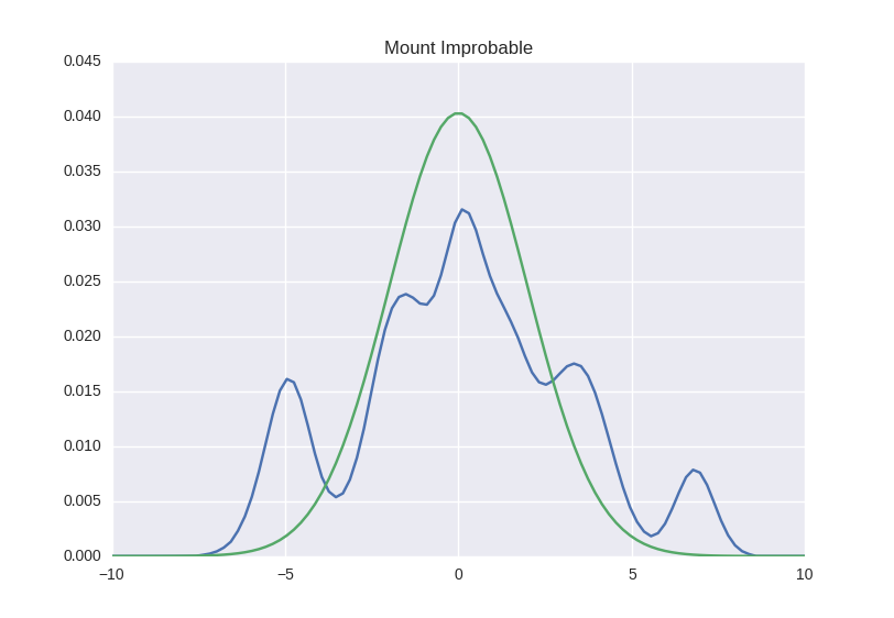
Well ... actually the devil knows. First of all, it’s not very clear yet, the approximation can be so accurate - it doesn’t look very much in the picture. Secondly, we do not yet know how to do this at all. So let's start and see.

Laplace approximation

Once again we will draw our Bayes theorem, just a little bit different:


I just collected the product of two probabilities to the right of the fraction into one - the so-called joint probability (and once again I remind you that we slightly changed the notation to w instead of theta). People often view it in the sense that - our "desired" distribution, and - the normalizing constant, which is needed to sum the result to one. So let's temporarily focus on searching. .

We say "approximation", remember the Taylor series . In accordance with the first course of mathematical analysis, any function is decomposed into an infinite sum of defined polynomials. We write our function as , and we will lay out at some point which coincides with the maximum distribution (we do not know where it is, but this is not important yet). And at the same time, we saw off an infinite sum after a term with a power of two:


(this is a straightforward one-to-one decomposition in a Taylor series from Wikipedia)

Now we remember that we have chosen as a point of maximum, and therefore, the derivative in it is zero. That is, the second term can be thrown out with a clear conscience. Get


Nothing like? In fact, this piece has the same shape as the logarithm from the Gaussian. To see this, you can write


Slightly change the notation: we wanted to choose and now let it be . Then and it turns out that our desired joint probability can be approximated by a Gaussian with a center at the maximum point and a standard deviation (inverse second derivative at the maximum point or curvature).

If it was too many incomprehensible symbols for one section, sum up the idea in three short paragraphs. So, if we want to find our volume of a mountain, we need:
- find the maximum point
- measure the curvature in it (calculate the second derivative; only attention: the derivative with respect to , but not )
- take a normal curve with a center at the maximum point and a standard deviation - negative-inverse to the curvature.

We are able to search for the maximum point of the mountain and it is much easier than measuring it all. Actually, let's apply magic to the same Bayes regression with which we worked in the last post!

We searched for the maximum point at the end of the last post — this is the center of the “Bayesian beam”, “the hottest line”, etc. I, just in case, once again give you how to find it, but I will hide it under the spoiler so as not to scare people with formulas:


Derivative by you can calculate it analytically, but since I'm a terrible bummer, I'd rather hammer all this into a python and let aurograd do the work for me.

# b  w       ,      #       ext_w = np.hstack([b, w]) #      #     ,  ext_data.dot(ext_w) #  data.dot(w) + b ext_data = np.ones((data.shape[0], data.shape[1] + 1)) ext_data[:, 1:] = data #   log joint,      #        def log_joint(w): regression_value = ext_data.dot(w) return ( np.sum(-np.power(target - regression_value, 2.) / (2 * np.power(1., 2.))) + np.sum(-np.power(w, 2.) / (2 * np.power(1., 2.))) ) from autograd import elementwise_grad second_grad_log_joint = elementwise_grad(elementwise_grad(log_joint)) mu = ext_w sigma = -1. / second_grad_log_joint(ext_w) cov = np.diag(sigma) # ,      # some_value = multivariate_normal.pdf(some_point, mu, cov)... 

When we have a distribution, drawing it is a matter of technique; We use approximately the same method as in the last part of the post with a slight modification (sample distribution at different distances from the center). We get just such a pretty picture:



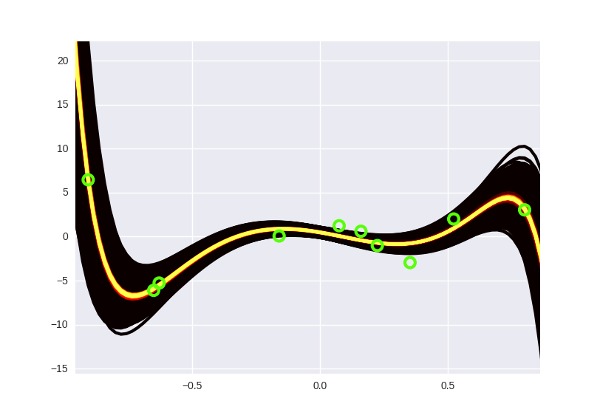
And by the way, each curve here is a 15 degree polynomial. The old “brute force” Bayes regression would have long since leaned back to lie down for several years of computer time (there I somehow squeezed the fifth degree).

The approximation of Laplace is good for everyone - quickly, conveniently, beautifully - but one thing is bad: it is estimated by the maximum point. This is how to judge all the grief, looking at it from the top - despite the fact that we do not know whether we are really on top or stuck in a local maximum, and despite what is far from all visible (suddenly we are very flat and beautiful, and under it three kilometers of a continuous cliff?). In general, they invented it for neural networks, as you might guess, not in the time of Laplace, but even in 1991, but since then it has not particularly won the world. So let's look at something more fashionable and beautiful.

Bayes by backprop: the beginning

Finally we got to that method from the heading article DeepMind. The authors called it Bayes by backprop - good luck with the translation into Russian, yeah. Reverse Bayesoraspread?

The starting point here is this: imagine that we have some kind of approximation (this is where the theta symbol came in handy - these will be our approximation distribution parameters), and let it be some simple form, also Gaussian, say. The trick is this: try to write down the expression of some “distance” from our approximation to the original mountain, and minimize this distance. Since both values ​​are probability distributions, we zayuzay thing, which was specially invented to compare distributions: Kullback-Leibler distance . In fact, it just sounds a little scary, and so this is just this:


If you carefully look at the integral, it becomes clear that it looks like a mathematical expectation - under the integral is some kind of thing multiplied by , and the integral is taken by . Then you can write it like this:


We go further: in the denominator we have , and we know that by the Bayes theorem it is . Put it in the formula above and note that under the expectation is - which does not depend on , and we can take it out of the expectations:


This we did a very cool thing. Because if you have not forgotten, this whole thing is equal to the difference between the approximation and our mountain. The controlled parameter here is , and we want to adjust it so that the difference is minimal. So, in the process of this minimization, we do not need to worry about
- because it does not depend on . And this, by the way, was the main problem component of our posterior - in order to calculate it, we just had to go around all the points of the mountain and put them together (because total for all , and there’s no other way to get it).

However, we go further. We are interested in finding the minimum of what is left:


How do we usually look for lows? Well, we take the derivative and make a gradient descent. Any idea how to get a derivative of this stuff? I still have something very.

Bayes by backprop: continued

Then comes the part in which I could not intuitively enter, so I have to glue my teeth and follow the math. The part that allows us to take a derivative is called reparameterization trick, and consists of the following steps:

1. Suppose we took some random variable . We don’t know anything about her, except that she’s chosen so that . Here is her property, and everything is about her.
2. Generally speaking, the derivative of the expectation is not as terrible as it seems: it is only a derivative of the integral, that is, roughly speaking, of the sum where the summation goes over . In and of itself, it is not scary, but tedious, because again we are returning to the problem called “pile up all the points of the infinitely growing ". Let's imagine in general terms that under the expectation of some kind of function , and write our derivative:

We did not do anything special - we just uncovered the expectation of Wikipedia by definition, recorded it again as an integral. But hey, see in the end? We just said it’s equal . And-iii ...


Now our integral is done by epsilon, which means we can drive the derivative with respect to
under the sign of the integral.


Here is the reparametrization trick: we had a derivative of the expectation, it was the expectation of the derivative. Cool? I suspect that if you are still following my slow finger movements along the lines, then you are not very cool, and maybe even not very clear what has changed - we need to integrate one FIG. What have we achieved at all?

The bottom line is that now we can approximate this integral at several points (samples). But before they could not. Previously, the derivative had to be taken from the entire amount: first to collect a bunch of points together, and then to differentiate it, and there any inaccuracy in collecting could lead us away when differentiating is far from the wrong direction. And now we can differentiate at points, and only then sum up the results - and this means that we can easily do with a partial sum.

These are the harsh orders in the world of approximate inference: here we need approximations in order to calculate the derivative , not even the posterior-distribution itself. Well, nothing, we are almost there.

Bayes by backprop: algorithm

Until now, we have been as abstract "parameters": it is time to clarify them. Let our approximation will be gaussian: then imagine as - average value, and - standard deviation. We also need to decide on - let's make it a Gaussian random variable with center at zero and standard deviation 1, i.e. . Then in order to fulfill the conditions for reparameterization, let


( here means elementwise multiplication). For me, however, it’s not very obvious why (if someone can explain on the fingers in the comments - I will be very grateful), but take this piece of article on faith.

In total, our reverse bayesoraspread consists of the following steps:

1. We start with random and for each neural net weight (or regression coefficient)
2. Sample a little of
3. We get from it
   
4. We recall our function of the distance between the "true mountain" and the approximation. We once designated it as but it is good . I'll write her below anyway , it's easier (keep in mind that ).
5. We consider the derivative with respect to . It will be:
   
   
   
   
   (where is the plus? because - a function of two variables, and both depend on )
   
6. We consider the derivative with respect to :
   
   
   
7. There are derivatives - it is figuratively wearing a hat. Next good old gradient descent:
   
   
   

Any results

I don’t know about you, but I’m already tired of this black and yellow bundle, so let's skip this mandatory stage and do something more like a neural network. The authors of the original article obtained nice results on MNIST-digits without any additional perversions such as using convolutional networks - let's try to get close to them. And perhaps it is time to put aside cute autograd to the side and arm yourself with something heavier like Theano. There will be a little bit of Theano-specific code, so if you are not targeting it, feel free to browse through it.

We get the data:

 from sklearn.datasets import fetch_mldata from sklearn.cross_validation import train_test_split from sklearn import preprocessing import numpy as np mnist = fetch_mldata('MNIST original') N = 5000 data = np.float32(mnist.data[:]) / 255. idx = np.random.choice(data.shape[0], N) data = data[idx] target = np.int32(mnist.target[idx]).reshape(N, 1) train_idx, test_idx = train_test_split(np.array(range(N)), test_size=0.05) train_data, test_data = data[train_idx], data[test_idx] train_target, test_target = target[train_idx], target[test_idx] train_target = np.float32(preprocessing.OneHotEncoder(sparse=False).fit_transform(train_target)) 

We declare the parameters. Here we apply a little trick, which is in the article, but I deliberately did not tell. The point is this: for each network weight, we have two parameters — mu and sigma, right? A small problem may arise from the fact that sigma must always be greater than zero (this is the standard deviation of the Gaussian, which cannot be negative by definition). First, how to initialize it? Well, you can take random numbers from something very close to zero (like 0.0001) to unity. Secondly, and if she does not stop in the process of gradient descent below zero? Well, it should not be like that, although at the expense of any arithmetic inaccuracies after the point, it can and. In general, the authors suggested solving this elegantly - we will replace sigma with the logarithm of sigma, and make the appropriate amendment to the weights formula:

(why is it under the logarithm +1? Apparently, with the same goal - in order not to accidentally take the logarithm from zero).

Oh, and we used to talk all the time about scales as , but we often have our own nomenclature in neural networks - zero weight, called there (bias). We will not break the agreement. So:

 def init(shape): return np.asarray( np.random.normal(0, 0.05, size=shape), dtype=theano.config.floatX ) n_input = train_data.shape[1] # L1 n_hidden_1 = 200 W1_mu = theano.shared(value=init((n_input, n_hidden_1))) W1_logsigma = theano.shared(value=init((n_input, n_hidden_1))) b1_mu = theano.shared(value=init((n_hidden_1,))) b1_logsigma = theano.shared(value=init((n_hidden_1,))) # L2 n_hidden_2 = 200 W2_mu = theano.shared(value=init((n_hidden_1, n_hidden_2))) W2_logsigma = theano.shared(value=init((n_hidden_1, n_hidden_2))) b2_mu = theano.shared(value=init((n_hidden_2,))) b2_logsigma = theano.shared(value=init((n_hidden_2,))) # L3 n_output = 10 W3_mu = theano.shared(value=init((n_hidden_2, n_output))) W3_logsigma = theano.shared(value=init((n_hidden_2, n_output))) b3_mu = theano.shared(value=init((n_output,))) b3_logsigma = theano.shared(value=init((n_output,))) 

This logsigm needs to somehow be able to cram it into the formula for a normal distribution, so we will do our function for it. At the same time and the usual declare:

 def log_gaussian(x, mu, sigma): return -0.5 * np.log(2 * np.pi) - T.log(T.abs_(sigma)) - (x - mu) ** 2 / (2 * sigma ** 2) def log_gaussian_logsigma(x, mu, logsigma): return -0.5 * np.log(2 * np.pi) - logsigma / 2. - (x - mu) ** 2 / (2. * T.exp(logsigma)) 

It is time to evaluate our probabilities. We do this, as we did before, by sampling - that is, we are spinning in a cycle, at each iteration we get a random-initializing epsilon, turn it into weights and put it together. In general, for the cycles in Theano there is a scan, but: 1) it was clearly developed by a team of manic inquisitors in order to break the brain of the user as much as possible and 2) for a small number of iterations, the usual cycle will fit us. Total:

 n_samples = 10 log_pw, log_qw, log_likelihood = 0., 0., 0. for _ in xrange(n_samples): epsilon_w1 = get_random((n_input, n_hidden_1), avg=0., std=sigma_prior) epsilon_b1 = get_random((n_hidden_1,), avg=0., std=sigma_prior) W1 = W1_mu + T.log(1. + T.exp(W1_logsigma)) * epsilon_w1 b1 = b1_mu + T.log(1. + T.exp(b1_logsigma)) * epsilon_b1 epsilon_w2 = get_random((n_hidden_1, n_hidden_2), avg=0., std=sigma_prior) epsilon_b2 = get_random((n_hidden_2,), avg=0., std=sigma_prior) W2 = W2_mu + T.log(1. + T.exp(W2_logsigma)) * epsilon_w2 b2 = b2_mu + T.log(1. + T.exp(b2_logsigma)) * epsilon_b2 epsilon_w3 = get_random((n_hidden_2, n_output), avg=0., std=sigma_prior) epsilon_b3 = get_random((n_output,), avg=0., std=sigma_prior) W3 = W3_mu + T.log(1. + T.exp(W3_logsigma)) * epsilon_w3 b3 = b3_mu + T.log(1. + T.exp(b3_logsigma)) * epsilon_b3 a1 = nonlinearity(T.dot(x, W1) + b1) a2 = nonlinearity(T.dot(a1, W2) + b2) h = T.nnet.softmax(nonlinearity(T.dot(a2, W3) + b3)) sample_log_pw, sample_log_qw, sample_log_likelihood = 0., 0., 0. for W, b, W_mu, W_logsigma, b_mu, b_logsigma in [(W1, b1, W1_mu, W1_logsigma, b1_mu, b1_logsigma), (W2, b2, W2_mu, W2_logsigma, b2_mu, b2_logsigma), (W3, b3, W3_mu, W3_logsigma, b3_mu, b3_logsigma)]: # first weight prior log_pw += log_gaussian(W, 0., sigma_prior).sum() log_pw += log_gaussian(b, 0., sigma_prior).sum() # then approximation log_qw += log_gaussian_logsigma(W, W_mu, W_logsigma * 2).sum() log_qw += log_gaussian_logsigma(b, b_mu, b_logsigma * 2).sum() # then the likelihood log_likelihood += log_gaussian(y, h, sigma_prior).sum() log_qw /= n_samples log_pw /= n_samples log_likelihood /= n_samples 

Fuh. Now we collect objective. Somewhere in this place in the post there should be a pause for two weeks, because the objective that is proposed in the article (something like (log_qw - log_pw - log_likelihood / M).sum() ) didn’t work for me and gave a very bad results. Then at some point I realized to finish the article to the end and found that the authors advise working with minibats and averaging the objective in a certain way. More precisely, even this:

 objective = ((1. / n_batches) * (log_qw - log_pw) - log_likelihood).sum() / batch_size 

At the same time advised to use the Adam optimizer instead of the usual gradient descent. I have never used it in my life, so we will resist the temptation to write it ourselves and use the ready-made one.

 from lasagne.updates import adam all_params = [ W1_mu, W1_logsigma, b1_mu, b1_logsigma, W2_mu, W2_logsigma, b2_mu, b2_logsigma, W3_mu, W3_logsigma, b3_mu, b3_logsigma ] updates = adam(objective, all_params, learning_rate=0.001) 

Well, then everything is standard - the train-function and go directly to learn. All code can be viewed here . A great percentage of accuracy is not there, it is true, but also the bread.

 epoch 0 cost 6.83701634889 Accuracy 0.764
 epoch 1 cost -73.3193287832 Accuracy 0.876
 epoch 2 cost -89.2973277879 Accuracy 0.9
 epoch 3 cost -95.9793596695 Accuracy 0.924
 epoch 4 cost -100.416764595 Accuracy 0.924
 epoch 5 cost -104.000705026 Accuracy 0.928
 epoch 6 cost -10.16.166556952 Accuracy 0.936
 epoch 7 cost -110.469004896 Accuracy 0.928
 epoch 8 cost -112.143595876 Accuracy 0.94
 epoch 9 cost -113.680839646 Accuracy 0.948

Leave the link to the article , just in case, once again, because there are a lot of interesting things there: how to move from approximation by Gaussians to something more complicated, or for example, how to use this thing in reinforcement learning (well, this is DeepMind, at the end all).

Q & A

1. There, in the article and in general everywhere, the word “variational” is often used, and nothing is said about it in the post.
   
   Here, to my shame, I was simply ashamed: at one time in school I didn’t have variational calculus, and I’m a little bit wary of using unfamiliar terms, especially since you can do without them. But in general, yes: you can read about the approach as a whole in the section on variational Bayesian methods . On the fingers, as I understand it, the meaning of the title is as follows: the calculus of variations works with functions in the same way as ordinary mathematical analysis with numbers. That is, where we in school were looking for the point at which the minimum of the function was achieved, here we are looking for the function (that ), which minimizes KL divergence, for example.
2. In the last post there was a question - what is the dropout and in general, is it somehow connected with the whole thing?
   
   And how. Dropout can be considered as a cheap version of Bayesian, but very simple. The idea is based on the same analogy with the ensembles, about which I mentioned at the end of the last post: now imagine that you have a neural network. Now imagine that you take it, accidentally tear off several neurons to it, and put it aside. After ~ 1000 such operations, you get an ensemble of thousands of networks, where each is slightly different from each other randomly. We average their predictions, and we find that random deviations in places compensate each other and give actual predictions. Now imagine that you have a Bayesian network, and you take out a set of its weights out of uncertainty a thousand times, and you get the same ensemble of slightly different networks.
   
   Than the Bayesian approach is cooler - it allows you to use this randomness in a controlled way. Look at the picture again: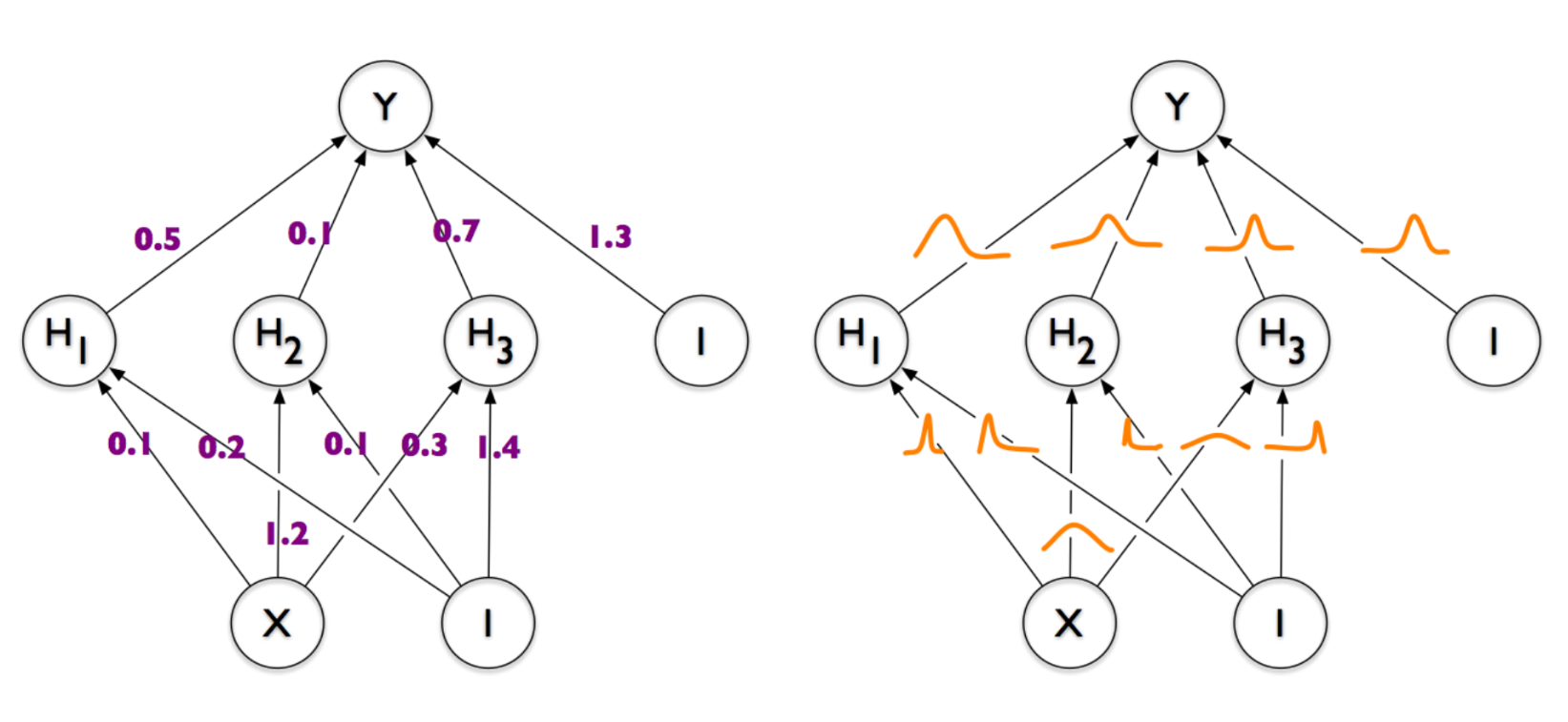
   
   
   
   Every weight here is a random variable, but these are different accidents. Somewhere the peak of the Gaussians is strongly shifted to the left, somewhere to the right, somewhere in the center and has a large variance. Presumably as a result of training, each weight acquires a form that is most suitable for the network to perform its task. That is, if we have some very important weight, for example, which must be strictly equal to something else, otherwise the whole network will break, then when sampling weights, this neuron will most likely remain in place. In the case of a dropout, we simply disconnect the weights evenly and randomly, and we can easily bang this important weight. Dropout does not know anything about its “importance”, for it all the weights are the same. In practice, this is reflected in the fact that the Dimpindov network produces better results than a network with a dropout, albeit only slightly.
   
   Than dropout steeper - this is because it is very simple, of course.
3. What do you do all this? Neural networks, presumably, must be built in the image of the thing in our head. There are obviously no Gaussian scales, but there are a lot of things that you machine operators ignore outright (time factor, discrete spikes and other biology). Throw out your textbooks on Terver and repent!
   
   A good way I like to think about neural networks includes the following historical chain:
   
   
   • people at some point thought that all thinking and processes in the world in general can be organized in a cause-effect chain. Something happened, then something else happened, and it all together affected something third.
   • they began to build such symbolic models such as ordinary Bayesian networks (not to be confused with the subject), and realized that such models could answer all sorts of different questions (“if it's sunny and Sebastian is happy, what is the likelihood that Sebastian was paid today?” ") And respond pretty well.
   • but in such models all variables had to be driven in by hands. At some point, connectionism came and said: let's just create a bunch of random variables and link them all together, and then somehow teach this model so that it works normally.
   
   And so it turned out including neural networks. They really should not be like the wet biological networks in our heads. They are made in order to get the right combination of causes and effects in the form of neurons, which are stuck one into another, somewhere inside them. Each neuron inside is a potential “factor”, some kind of variable responsible for something, and Bayesian magic helps to make these factors more useful.
   
   What does every neuron inside our head do? Hell knows. It may well be that nothing special.
4. What else is on this topic?
   
   Oh, a lot of things:
   
   
   • Variational autoencoders - in my opinion, almost the most popular model, and in an amicable way, it was necessary to start with it, but I really liked this one.
   • In fact, if you look a little deeper into the history of machine learning, then variational approximations stick out of each iron there. Say, in the deep Bolztmann machine (which are not particularly used anywhere, it seems, but enive), or in a piece called NADE , which remakes the Boltzmann machine in the language of the reverse propagation of an error.
   • Variational black box - I do not even know what it is, because I stumbled upon it only when writing a post, but I already like the name and the promise in the introduction.
   • DRAW , which I can’t get to in any way and which looks simply amazing: a recurrent network with attention-mechanism that can draw digits like a pencil.
   • a thing called Ladder Network that combines supervised and unsupervised learning