Genetic Programming ("Yet Another Bicycle" Edition)

Let's take a break from the next "killer language C ++", stunning synthetic performance tests of some NoSQL database engine, HYIP around the new JS framework, and dive into the world of "programming for programming".
Foreword
March began for me with reading articles about the fact that Habr is no longer a cake . Judging by the response, the topic was opened sore. On the other hand, I managed to learn something for myself from this: "you are the Resistance" if you read this - you are Habr. And to make it more interesting (or at least more diverse, to move away from the emerging trend of aggregation of advertising posts, around-line and corporate blogs) is possible only by ordinary users. I just had a small project at that time, although it required serious improvement, which I wanted to tell about. And I decided - for a month ( naive! ) I will write an article. As we can see, now the middle end of april early may May is in full swing, you can blame both my laziness and the irregularity of free time. But still, the article saw the light! What is interesting, while I was working on the article, two similar ones had already come out: What is grammatical evolution + easy implementation , Symbolic regression and another approach . If I were not so slow, it was possible to fit in and declare a month of genetic algorithms :)
Yes, I fully realize that it is 2016, and I write such a long post. More and drawings are made in the style of "chicken paw" pen on the tablet, with fonts Comics Sans for geeks xkcd .
Introduction
Some time ago an interesting article appeared on GT, with, which is characteristic, even more interesting comments (and what kind of verbal battles were there about natural selection!). There was a thought that if we apply the principles of natural selection in programming (to be more precise, in metaprogramming )? As you can guess, this thought eventually led me to the re-discovery of the long-existing concept of genetic algorithms . Having quickly studied the hardware, I enthusiastically rushed to experiment.
But let's get everything in order.
')
Likbez
Virtually all the principles underlying genetic algorithms are derived from natural, natural selection — populations adapt to environmental conditions through a change of generations, and the most adapted ones become dominant.
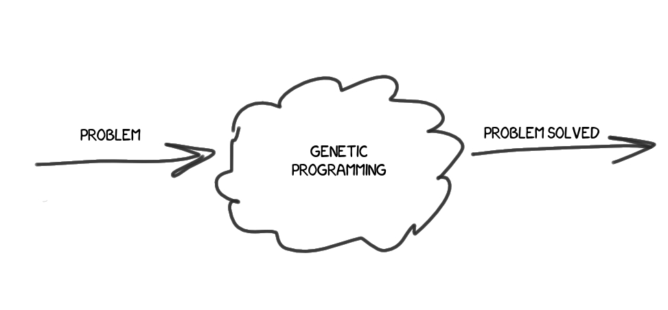
How to solve problems using genetic algorithms? You will be surprised how everything just works in the zero approximation:
Now WE NEED TO GO DEEPER . First approach:
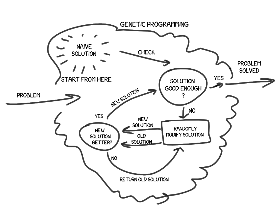
So, we have a problem / problem, we want to find its solution. We have some basic, poor, naive solution, the results of which, most likely, do not satisfy us. We will take the algorithm of this solution and slightly modify it. Naturally random, without analytics, without understanding the essence of the problem. A new solution was to give the result at least a little better? If not - discard, repeat again. If yes - hooray ! Does the result of the new solution fully satisfy us? If yes - we are great, solved the problem with a given accuracy. If not, take the resulting solution and perform the same operations on it.
Here is a brief and unsophisticated description of the idea as a first approximation. However, I think it will not satisfy inquiring minds.

For starters, how do we modify solutions?
Our solution consists of a set of discrete blocks - characteristics, or, if you please, genes. Changing the set, we change the solution, improving or worsening the result. I depicted the genotype as a chain of genes, but in practice it will be a tree structure (not excluding, however, the ability to contain a chain in one of its nodes).
Now let's consider the main loop in more detail:
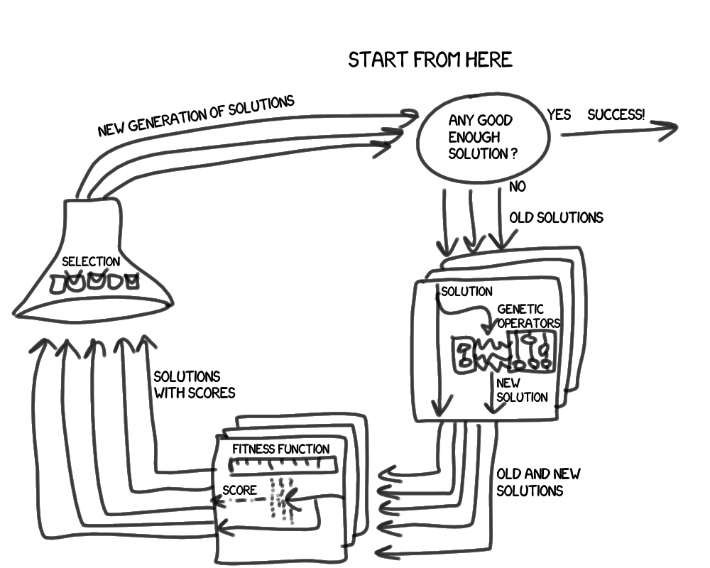
What became distinguishable in the second approximation? First, we operate not with one, but with a group of decisions, which we will call a generation . Secondly, new entities have appeared:
- Genetic operations (yes, the eternal confusion with the translation, the English " operator " is our " operation ") are needed to get a new solution based on the previous ones. This is usually a crossing (random combination of two different solutions) and mutation (random change of one solution).
- The fitness function (I liked the fitness function more ) is needed to assess the degree of our satisfaction with the result of the decision.Who comes to mind TDD?Indeed,
whenif we learn how to easily write tests that answer not only the question of whether our code is flooded with a test or not, but also give a measurable assessment of how close it has come to success , we will be one step closer to self-written programs. Do not be surprised if such attempts have already been. - Breeding describes the principles of selection decisions in the next generation.
disadvantages
No matter how promising it may sound, the approach to solving problems under discussion is complete. fatal fundamental flaws. While practicing, I stumbled over, probably, about all the known pitfalls. The most important, in my opinion, of them: poor scalability. The growth rate of the cost of computation on average exceeds the growth rate of the input data (as in the naive sorting algorithms). On the other shortcomings, I will tell you along the way.
Practice
Language selection
Ruby was chosen. This language filled a niche in my affairs, which traditionally occupied Python, and it fascinated me so much that I certainly decided to get to know him better. And here is the opportunity! I like to kill N (where N > 1) hares at a time. I do not exclude that my code may sometimes cause smiles, if not the old Rubists' feyspalms (no, sorry, but it is the UBist , the other options are trolling).
Genotype
The first thought was that once there is an eval in the language, then the genotype of the solution can be built without any tricks of arbitrary characters (acting as genes), and we will have a script interpreted by Ruby as a result. The second thought was that the evolution of solutions with such high degrees of freedom can actually take many years. So I did not even lift a finger in this direction, and I think I did not lose. You can try this approach in about 30 years if Moore's law is preserved.
Evolution in the end was enclosed in a fairly rigid framework. Solution genes are highly organized tokens with the possibility of nesting (building a tree structure).
In the first experiment, where we will talk about solutions as mathematical expressions, tokens are constants, variables, and binary operations (I don’t know how legitimate the term is, in the context of the project "binary operation" means action on two operands, for example, addition).
By the way, I decided to partially leave compatibility with eval , so if I request a string representation of the token (via standard to_s ), then I can get a completely digestible string for interpretation. For example:
f = Formula::AdditionOperator.new(Formula::Variable.new(:x), Formula::IntConstant.new(5)) f.to_s # "(x+5)" Yes, and more clearly so.
Genetic operations
As the main and only way to change the genotype of solutions, I chose a mutation . Mainly because it is easier to formalize. I do not exclude that breeding by crossing could be more effective (and judging by the example of living nature, it seems to be so), but in its formalization many pitfalls are hidden, and, most likely, certain restrictions are imposed on the very structure of the genotype. In general, I went the easy way.
In the sections of the article devoted to the description of final experiments, the rules for mutation of solutions are described in detail. But there are common features that I want to talk about:
- Sometimes (in fact, often) it happens that in just one step of a mutation it is impossible to achieve improved results, although the mutation goes, in general, in the right direction. Therefore, in the phase of applying genetic operations, solutions are allowed to mutate an unlimited number of times per turn. The probability looks like this:
- 50% - one mutation
- 25% - two mutations
- 12.5% - three mutations
- etc. - It happens that in a few steps a mutant can become identical to a parent, or different parents get the same mutants; such cases are stopped. Moreover, I decided to maintain the strict uniqueness of decisions within a single generation.
- Sometimes mutations give rise to completely unworkable solutions. It is extremely difficult to deal with this analytically; usually, the problem is revealed only at the moment of their assessment by the fitness function. I allow such decisions to be. All the same, most will disappear over time as a result of selections.
Fitness function
There are no problems with its implementation, but there is one caveat : the complexity of the fitness function grows almost on a par with the increase in the complexity of the problem being solved. So that she was able to do her job within a reasonable time, I tried to implement it as simply as possible.
Recall that the generated solutions return a specific result based on a specific set of input data. So, it is implied that we know what an ideal ( reference ) result should be obtained for a certain set of input data. The results are quantifiable, which means we are able to quantify the quality of a particular solution by comparing the returned result with the reference one .
In addition, each solution has indirect characteristics, from which I selected, in my opinion, the main one - resource intensity. In some tasks, the resource consumption of a solution is dependent on the input data, while in others it is not.
Total fitness function:
- calculates how much the results of the solution differ from the reference
- determines how resource-intensive the solution
In early prototypes, I tried to measure the processor time spent on testing, but even with long (tens of milliseconds) runs, there was a variation of ± 10% of the time on the same solution introduced by the operating system, with periodic emissions + 100-200%.
So in the first experiment, the resource intensity is calculated by the total complexity of the genotype, and in the second calculation, the actually executed code instructions
Selection
Each generation contains no more than N solutions. After applying genetic operators, we have a maximum of 2N solutions, and no more than N of them will pass to the next generation.
What is the principle behind the next generation of solutions? We are at a stage when each of the solutions has already received an assessment of the fitness function. Estimates, of course, can be compared with each other. Thus, we can sort the current generation of solutions. Then it seems logical to simply take the X best solutions, and form the next generation of them. However , I decided not to dwell on this, and to include in the new generation also Y random solutions from the rest.
For example, if X = Y , then to decide to go to the next generation, he needs to be among the 25% of the best, or throw 3 on a three-sided dice (if such existed). Enough humane conditions, right?
So, the inclusion of accidental survivors in the next generation is necessary to preserve the species diversity. The fact is that for a long time those who keep among the best similar solutions squeeze out the rest, and the further, the faster the process, and in fact it often happens that the dominant branch turns out to be a dead end.
Parameters X and Y , of course, are customizable. I ran tests with and without random survivors, and proved the validity of adding them to the algorithm: in some cases (when searching for solutions of increased complexity), I managed to achieve better results with their use (moreover, the total power spent on searching for solutions constant, for example, X 1 = 250, Y 1 = 750 against X 2 = 1000, Y 2 = 0).
Victory conditions
Here lies the catch: how to understand what time to finish? Suppose the solution satisfies us in terms of the accuracy of the results, but what about the complexity? Suddenly, the algorithm will now work and produce a solution for coloring graphs in O (n) ? I exaggerate of course, but the criterion for stopping work needs to be formalized. In my implementation, the execution of the algorithm ends when Top 1 solution does not change a certain number of generations (abbreviated R -rounds). The lack of rotation means that, firstly, there was no alternative solution that could outperform the best current solution; secondly, the best current solution failed to produce an improved mutation of itself for a given time. The number of generations through which the victory of a better solution comes is usually a large number — to really make sure that evolution is not able to go any further, a change of several hundred (the number varies depending on the complexity of the task itself) of generations is required.
Unfortunately, despite numerous precautions, there are cases when evolution comes to a standstill. This is a well-known problem of genetic algorithms, when the main population of solutions focuses on the local optimum , ignoring, as a result, the desired global optimum . This can be answered with a game with parameters: a decrease in the quota for the winners, an increase in the quota for random, and an increase in the time of dominance for the victory, parallelization of independent generations. But all this requires power / time.
Concrete implementation
As is customary, everything is laid out on a githab (admittedly, without docks yet).
Now that we will see in specifically my bike ride implementation:
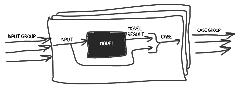
- Introduces the concept of reference (Model). We treat it as a black box, with which, based on the input data (Input), you can get a reference result (Model Result).
- Case (case) simply contains a set of input data and a reference result.
We collect a set of cases (Case group) on the basis of a set of input data (Input group).
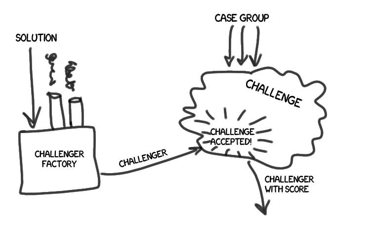
- A challenge (or trial ) (Challenge) is a set of actions for completing a set of cases formed earlier. On the shoulders of the test also work on the evaluation of the results of the passage, and comparison of assessments.
We have a challenger (Challenger), which has a certain solution (Solution). The challenger makes a sacramental
" challenge accepted! ", And learns his degree of fitness (Score).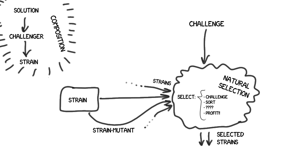
- As a result, we build a chain of composition - a solution (Solution - provides a solution to a specific type of problem) -> challenger (Challenger - is being tested ) -> strain (Strain - participate in natural selection and evolution (see below))
There is a natural selection (Natural Selection), which includes the test , and filters the group of strains coming to it according to specified rules.
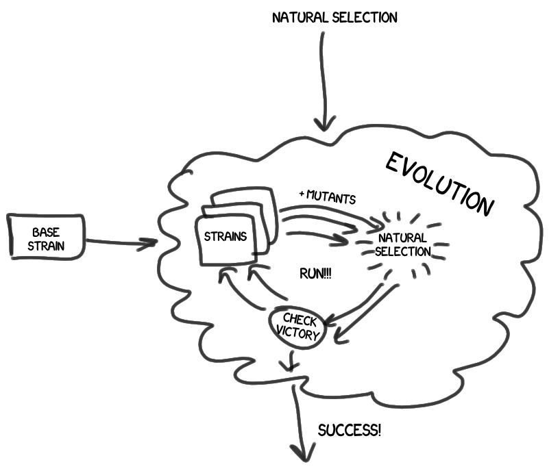
- At the top level is evolution (Evolution), which, including natural selection , controls the entire life cycle of the strains.
- The result of the evolutionary work is a winning strain, which we honor as a hero, and then we carefully study it, including its pedigree. And we draw conclusions.
Such is my general implementation of the genetic algorithm. At the expense of abstract classes (in Ruby , aha> _ <), we managed to write a code that was generally independent of a specific task area.
In subsequent experiments, the necessary Input, Model, Solution, Score (which, of course, quite a lot) were added.
Experiment One: Formulas
Generally, it would be more accurate to call Experiment One: Arithmetic expressions , but when I chose a name for the base class of expressions, then, without thinking twice, I stopped at Formula , and in the article I will call arithmetic expressions formulas . In the experiment, we introduce the formula-standards (the same Model ), containing one or several variables. For example:
x 2 - 8 * x + 2.5
We have a set of variable values ( Input Group , aha), for example:
- x = 0;
- x = 1;
- x = 2;
- ....
- x = 255;
Solutions ( Solutions ), which we will compare with the standards , are the same formulas, but created by chance - consistently mutated from the basic formulas (usually just x ). The score of the quality of the decision is the average deviation of the result from the result of the standard , plus the resource intensity of the solution (the total weight of the operations and the arguments of the formula).
Formula Mutation
As mentioned earlier, tokens of formulas are constants, variables, and binary operations.
How is the mutation of formulas? It affects one of the tokens contained in the formula, and can go in three ways:
- grow - growth, complication
- shrink - reduce, simplify
- shift - modification with conditional preservation of complexity
Here is a table of what happens with different types of formulas for different types of mutations:
| Formula → Mutation ↓ | Constant | Variable | Binary operation |
|---|---|---|---|
| grow | becomes a variable, or is included in a new random binary operation (with a random second operand) | to a new random binary operation (with a random second operand) | included in a new random binary operation (with a random second operand) |
| shrink | impossible to reduce, so we apply the shift operation to it | becomes constant | instead of the operation, only one of the operands remains |
| shift | changes its value to a random value, can change the type (Float <-> Int) | becomes another random variable (if it is allowed in this context) | either operands are reversed, or the type of operation is changed, or an attempt is made to reduce the operation |
Note 1. Reduction of formulas is an attempt to perform operations on constants in advance, where possible. For example, from " (3+2) " get " 5 ", and from " 8/(x/2) " get " (16/x) ". The task unexpectedly turned out to be so nontrivial that it forced me to write a prototype solution with an exhaustive unit test , and I didn’t achieve a real recursive solution, which yielded constants for reduction from any depth. It was fascinating to understand this, but at some point I had to stop myself and confine myself to the solution reached, because I was too deviated from the main tasks. In most situations, the reduction and so fully works.
Note 2 The mutation of binary operations has a peculiarity, due to the fact that operations have other formulas enclosed in themselves - operands. To mutate both the operation and the operands is too big a change for one step. So it is randomly determined which event will occur: the binary operation itself mutates with a 20% probability, the first operand mutates with a 40% probability, and with the remaining 40% probability, the second operand mutates. I can not say that the ratio of 20-40-40 is ideal, perhaps we should introduce a correlation between the probability of operation mutation depending on their weights (in fact, the nesting depth), but so far it works like this.
results
Now for the sake of which, in fact, everything was started:
The first standard is a simple polynomial:
x 2 - 8 * x + 2.5
X takes values from 0 to 255, in increments of 1
R = 64, X = 128, Y = 128
Runs are performed three times, here is the best result of the three. (Usually, all three times give identical results, but occasionally it happens that mutations come to a standstill and cannot even achieve a given accuracy)
The results struck me to the heart :) For 230 (including those R times when Top 1 did not change) the following decision was made for the generations:
(-13.500 + ((x-4) 2 ))Complete pedigreeAs you remember, more than one mutation is allowed between one generation.x (x-0) ((x-0)-0.050) (0.050-(x-0)) (0.050-(x-1)) (x-1) (x-1.000) ((x-1.000)--0.010) ((x-1.000)-0) ((x-1.000)-(1*0.005)) ((x-1.000)/(1*0.005)) ((x-1.020)/(1*0.005)) ((x-1.020)/(0.005*1)) ((x**1.020)/(0.005*1)) ((x**1)/(0.005*1)) ((x**1)/(0.005*(0.005+1))) ((x**1)/(0.005*(0.005+1.000))) (x**2) ((x--0.079)**2) ((x-0)**2.000) (((x-0)**2.000)/1) (((x-0)**2)/1) ((((x-0)**2)-0)/1) (((x-0)**2)-0) (((x-0)**2)-0.000) (((x-(0--1))**2)-0.000) (((x-(0--2))**2)-0.000) (((x-(0--2))**2)+0.000) (((x-((0--2)--1))**2)+0.000) (((x-((0--2)--1))**2)+-0.015) (((x-((0--2)--1))**2)+0) ((-0.057+0)+((x-((0--2)--1))**2.000)) ((-0.057+0)+((x-3)**2.000)) (((-0.057+0)**-1)+((x-3)**2.000)) (((-0.057+0)**-1)+((x-4)**2.000)) (((-0.057+0)**-1.000)+((x-4)**2.000)) (((-0.057+0.000)**-1.000)+((x-4)**2.000)) (((x-4)**2.000)+((-0.057+0.000)**-1.000)) (((x-4)**2)+((-0.057+0.000)**-1.000)) (((x-4)**2)+((-0.057+0.000)**-0.919)) ((((x-4)**2)+((-0.057+0.000)**-0.919))+-0.048) ((((-0.057+0.000)**-0.919)+((x-4)**2))+-0.048) ((((-0.057+0.000)**-0.919)+((x-4)**2))+-0.037) (((-0.057**-0.919)+((x-4)**2))+-0.037) (-0.037+((-0.057**-0.919)+((x-4)**2))) (-13.524+((x-4)**2)) (-13.500+((x-4)**2))
That is, after the results of the calculations finally began to coincide with the reference ones, he pursued resource-intensiveness, and carried out the transformations, and as a result, the formula based on natural selection wins in compactness!
It is curious that I got this result, in fact, by mistake. At the first runs, the types of mutations were prohibited, under which one more variable x would be added. Oddly enough, it worked even better than with a full mutation. Here are the results when the bug was fixed:
- R = 250, X = 250, Y = 750, Accuracy = 0.001, ( weight of result 49)
(2,500 + ((x-8) * x))
- R = 250, X = 1000, Y = 0, Accuracy = 0.001, ( weight of result 60)
(((x-1) * (- 7 + x)) - 4,500)
In this case, the option with a quota for random stumbled once, but still managed to produce a more optimal result than the second option, which each of the runs went through exactly and uniformly. Here, for each approximation of the result to the optimum, one mutation step is basically enough. In the next case, it will not be so easy!
The second standard is the natural logarithm:
ln (1 + x)
x takes values from 0 to 25.5, in increments of 0.1
Our solutions are unable to use logarithms directly, but this benchmark is decomposed into a Taylor series:
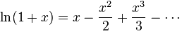
So let's see if the solution can reproduce such a series with a given accuracy.
At first, I tried the runs with an accuracy of 0.001, but after several days of hard work of the algorithm, the solutions reached an accuracy of only about 0.0016, and the size of the expressions was aimed at a thousand characters, and I decided to lower the precision bar to 0.01. The results are as follows:
- R = 250, X = 250, Y = 750, Accuracy = 0.01, (result weight 149)
((((-1.776-x) /19.717) + (((x * x) -0.318) ** 0.238)) - (0.066 / (x + 0.136))))
- R = 250, X = 1000, Y = 0, Accuracy = 0.01, (result weight 174)
(((-0.025 * x) + (((x * x) ** 0.106) ** 2)) / (1+ (0.849 / ((x * x) +1)))))
As you can see, in the case of the inclusion of random survivors for this standard, a less resource-intensive solution was found, while maintaining the specified accuracy. Not that it is very much like the Taylor series, but it believes true :)
The third standard is the sine, given in radians:
sin (x)
x takes values from 0 to 6.28, in increments of 0.02
Again, the standard is decomposed into a Taylor series:
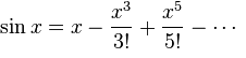
In this case, given that for any x, the result takes a value from -1 to 1, the detection accuracy of 0.01 was a more serious test, but the algorithm coped.
- R = 250, X = 250, Y = 750, Accuracy = 0.01, (result weight 233)
((((-0.092 ** x) /2.395) + (((- 1.179 ** ((((x-1) * 0.070) + - 0.016) * 4.149)) - (0.253 ** x)) + 0.184 )) ** (0.944- (x / -87)))
- R = 250, X = 1000, Y = 0, Accuracy = 0.01, (result weight 564)
(((x + x) * ((x * -0.082) ** (x + x))) + (((x + x) ** (0.073 ** x)) * ((((1 - (- 0.133 * x)) * (- 1-x)) * ((x / -1) * (- 0.090 ** (x - 0.184)))) (((((- 1.120+ (x * ( x + 1) * - 0.016))) ** (- 0.046 / ((0.045 + x) ** - 1.928))) + (- 0.164- (0.172 ** x))) * 1.357) ** 0.881)) ))
Again, due to the increased complexity of the standard, the best result was achieved by the version of the algorithm with a pool of random solutions.
The fourth benchmark is an expression with four (coincidence? I don’t think) variables:
2 * v + 3 * x - 4 * y + 5 * z - 6
Each of the variables takes values from 0 to 3 in increments of 1, for a total of 256 combinations.
- R = 250, X = 250, Y = 750, Accuracy = 0.01, ( weight of result 254)
((y * 0.155) + (- 2.166 + (((((z * 4) - (((y- (x + (y / -0.931))) * 2) + - 0.105)) + ((v + (v -2)) + - 0.947)) + x) + (z + -1)))))
- R = 250, X = 1000, Y = 0, Accuracy = 0.01, (result weight 237)
((-3 + (v + z)) + (((v + ((xy) + ((((z + z) - (((0.028-z) -x) + (y + y))) - y ) + z))) + x) + - 2.963))
Contrary to my expectations, the complexity of the compared with the first benchmark jumped very seriously. It seems that the standard is not difficult, you can safely step by step build up the solution, bringing the result to the desired one. However, the accuracy of 0.001 was never mastered! Then I began to suspect that the problems with scaling tasks in our approach are serious.
Results
In general, I was more likely not satisfied with the results obtained, especially with reference to standards 2 and 3. It took thousands of generations to eventually bring out cumbersome formulas. I see three options why this happens:
- An imperfect reduction mechanism — for example, a more far-sighted disclosure of brackets / brackets is missing. Because of this, the formulas do not result in a comfortable look.
- Too spontaneous mutation, and, the larger the formula, the less likely the correct further development. I was thinking about creating a "exhaustive" mechanism of mutation when a group of conditionally all possible mutants is formed on the basis of the original, and a pre-selection is made on it. Whether the hands reach to test the guess, whether this will improve the algorithm is still unknown.
- The principal impracticality of such a method for finding solutions to complex problems. Perhaps this approach is not so far gone from attempts to write "War and Peace" by forces of the army of monkeys with typewriters . Perhaps complexity, the need for an analytical approach, is a natural and inalienable property of such tasks.KurezI remembered how ten years ago I was interested in data compression, tried my hand at writing my own solution. He lamented that I could not compress random patterns at all until I was enlightened :) Maybe this is the case?
Further experiments
, .
, (, , ) ( , "" ""), , .
— . . , : - , , .
, ? . , , ? ,
nil — ? .
, , , — , . , - .
, .
. !
Source: https://habr.com/ru/post/279813/
All Articles