About one funny approach to filtering unimodal signals
In this article, our engineers would like to share with Habr a rather interesting tool that can be effectively used to filter out noisy signals, using a priori knowledge of signal unimodality.
The problem of offline signal filtering in the case when the expected waveform is known with an accuracy of up to several unknown parameters is reduced to the approximation problem. For example, if it is known that the signal grows linearly over the considered interval, the problem will be reduced to linear regression, and if it can be assumed that the noise is normal, then the correct method will be OLS . But once we faced the task of evaluating the shape of an X-ray microprobe profile (beam), about which only one thing was known a priori: the profile is unimodal, namely, it has exactly one maximum. It turns out that in this case, the best (in the sense, for example, L2 metrics) approach the experimental signal with a function belonging to a known set (a set of unimodal functions). Moreover, with acceptable asymptotics of computational complexity.
 ===>
===>  ===>
===> 
So, we will talk about the problem of approximation of a certain noisy signal as functions of a discrete argument
  , and it is known that the original signal is unimodal. In the case under consideration, it is additionally known that at the edges the signal asymptotically approaches zero. It should be noted that the method considered below does not in itself require such an assumption.
')
First, for simplicity, it makes sense to consider the same problem for a monotonic function. The description is given for a monotonously non-strictly increasing function, although, of course, for the monotonically decreasing one can do the same.
If we assume that the noise is normally distributed, then the problem will be reduced to minimizing the quadratic functional%20-%20Y(X_i))%5E2%7D) in the presence of inequalities of the form
in the presence of inequalities of the form %20%5Cge%20%5Cwidetilde%7BY%7D(X_i)) . This is a quadratic programming problem, and for it on the Internet you can find a number of ready solvers. But, first, the problem of quadratic programming in the general case is calculated rather slowly, and secondly, the problem of approximating a unimodal signal is not written out in a similar form if the position of the extremum is not known in advance.
. This is a quadratic programming problem, and for it on the Internet you can find a number of ready solvers. But, first, the problem of quadratic programming in the general case is calculated rather slowly, and secondly, the problem of approximating a unimodal signal is not written out in a similar form if the position of the extremum is not known in advance.
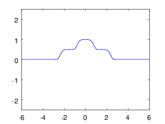
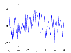
There is an alternative solution that does not have these disadvantages, but when using it, the signal scale will have to be considered discrete. It is worth noting that the task is not interesting in the case of low noise, since the usual linear filtering will most likely remove all practical problems. What is interesting, strong noise? In fig. 1, one can see a model signal before and after such a noise. The noise here is given by a normal distribution.
 ) . Under such conditions, the discretization of the approximating signal does not seem to be a significant loss. In addition, as will be seen later, as the number of samples increases, the complexity of the calculations will increase linearly.
. Under such conditions, the discretization of the approximating signal does not seem to be a significant loss. In addition, as will be seen later, as the number of samples increases, the complexity of the calculations will increase linearly.

Fig. 1: a) Model monotonous signal until the noise increases. b) Model monotonous signal after noise imposing.
It turns out that in the discrete approximation, filtering a normally noisy monotone signal reduces to dynamic programming with two parameters, and using this solution, it is possible to construct a computational circuit of the same complexity for a unimodal case.
You can read about what dynamic programming is here , and how and to which tasks it is used - here .
In the problem under consideration, the dynamic programming table is two-dimensional, its columns i correspond to increasing values of the discrete argument from left to right experimental points, and lines j - increasing from the bottom up possible values of the approximating function . Minimized functional - the sum of squared deviations from along paths with allowable crossings. It is obvious that the transitions to 1 to the right with a simultaneous non-negative upward shift will be admissible.
The outer loop is conducted along the coordinate i from left to right. For each value an inner loop is performed on the j coordinate from bottom to top. The minimum value of the functional is determined by the formula
%20%2B%20(Y_j%20-%20%5Cwidetilde%7BY%7D_j)%5E2%2C%0A)
and outside the table, the functionality is considered to be zero.
At the same time, in order not to recalculate each time the minimum at smaller values of j , it is useful to save it during the filling process along with the value of the functional, and since at the end you need to restore the path, it is more convenient to save the value of m at which this minimum was reached:

Then the calculation of the functional itself can be performed in O (1) for each cell:
%5E2.%0A)
After the completion of the direct passage, it remains to obtain an approximation in an explicit form. To do this, look for a minimum among the values of the functional for the rightmost column (the column with the highest coordinate i ), and then perform a reverse pass through i , with the index being restored, the value of the filtered signal j * in each column:
%2C%20%26%20i%20%3D%20n%20-%201%20%5C%5C%0Am_%7Bi%2Cj%5E*_%7Bi%2B1%7D%7D%2C%20%20%20%20%20%20%20%20%20%20%20%20%20%20%20%20%20%20%20%20%20%20%20%20%20%20%20%20%20%20%20%20%20%20%20%20%20%20%20%20%26%20i%20%3C%20n%20-%201%0A%5Cend%7Bcases%7D%0A)
Final values defined as
%20%3D%20%5Cwidetilde%7BY%7D_%7Bj%5E*_i%7D%0A)
In fig. 2 shows an example of the result of the described algorithm for a monotonous signal.
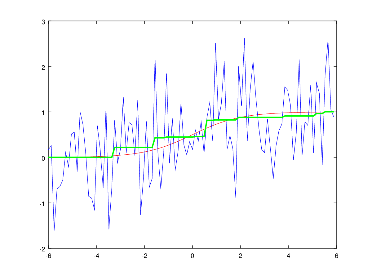
Fig. 2: Filtering a monotonically increasing signal by dynamic programming. The input noise signal is shown in blue, the result of the algorithm is shown in green, the ideal non-noise signal in red.
On this consideration of the auxiliary monotonous case is completed.
Using the result obtained, one can solve the problem of a unimodal signal by filling in 2 tables of the DP: one is filled as for a monotonic function, the second - in the same way, but in the opposite direction. As a result, 2 functionalities are calculated: and
and  as well as values
  and
and  to restore paths to tables. After that, among all values of i and j, such a pair is searched.
 ) for which the sum of the functionals is minimal is the indices of the maximum of the approximated function. The values of the function on each side of it are restored according to the corresponding table.
for which the sum of the functionals is minimal is the indices of the maximum of the approximated function. The values of the function on each side of it are restored according to the corresponding table.
%20%3D%20%5Coperatornamewithlimits%7Bargmin%7D%5Climits_%7Bi%2C%20j%7D(W%5E%7Blr%7D_%7Bi%2C%20j%7D%20%2B%20W%5E%7Brl%7D_%7Bi%2C%20j%7D)%0A)

Figures 3 and 4 show an example of the original unimodal signal and the result of its processing by the proposed algorithm.

Fig. 3: Noisy unimodal signal.
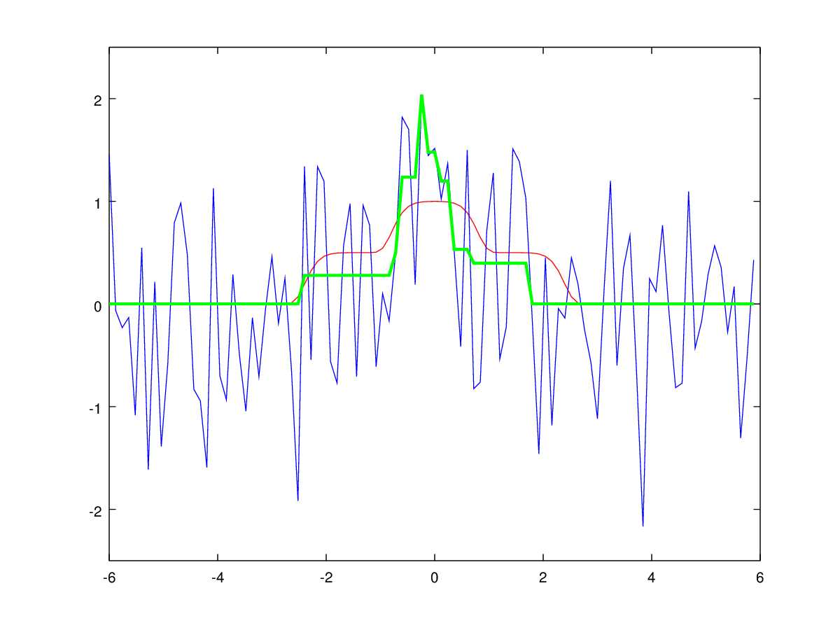
Fig. 4: Filtering a unimodal signal by dynamic programming. The input noise signal is shown in blue, the result of the algorithm is shown in green, the ideal non-noise signal in red.
In case it is known that the signal cannot change faster than some fixed speed (which is quite likely), the accuracy of the regression can be improved by introducing this restriction into the algorithm explicitly. To do this, it is enough to calculate the maximum possible change in the signal value index
  for each i and prohibit transitions in the DP table with a change in j by more than this value:
%20%2F%20(%5Cwidetilde%7BY%7D_%7B1%7D%20-%20%5Cwidetilde%7BY%7D_%7B0%7D)%5Crceil%0A)
%20%2B%20(%5Cwidetilde%7BY%7D_%7Bj%7D%20-%20Y_%7Bj%7D)%5E2%0A)
However, in order not to lose in laboriousness, you need to be able to get the minimum value of the functional on the segment [ j - dj , j ] for a constant time.
This can be done using the Van Herk-Gil-Verman algorithm, described, for example, here .
The result of applying the algorithm with the restriction on the derivative shown in fig. five.
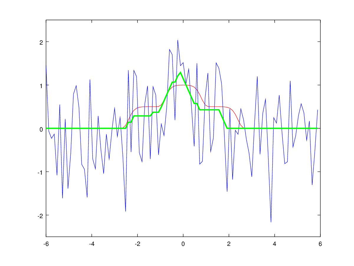
Fig. 5: Filtering a unimodal signal by dynamic programming with a limitation on the rate of change of the signal. The input noise signal is shown in blue, the result of the algorithm is shown in green, the ideal non-noise signal in red.
An inquisitive reader may suspect that the same or better results can be achieved in simpler ways. Of course, with certain parameters of the signal and noise, the described technique will be superfluous. In addition, the road you know is shorter. Therefore, for each tricky case a specialist will surely find a favorite method that will give an acceptable result in his hands.
To dispel a sense of possible fraud, in fig. Figures 6 and 7 show examples of signal processing by Gaussian smoothing and median filtering with a zerkalization at zero. Filter parameters were selected in order to obtain an optimal result, but without fanaticism.
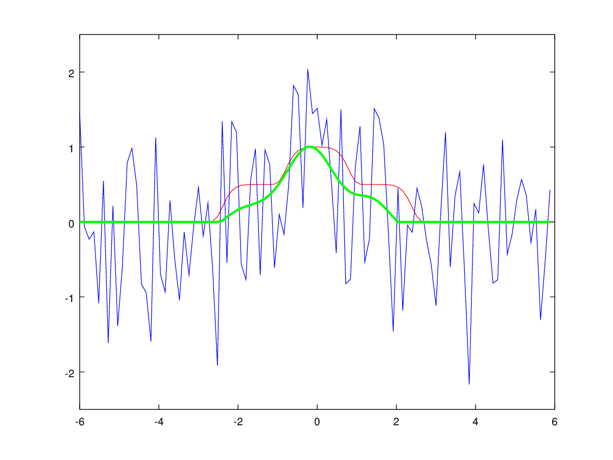
Fig. 6: Filtering a unimodal signal with Gaussian smoothing. The blue color shows the input noisy signal, green - the result of filtering, red - the ideal non-noise signal.
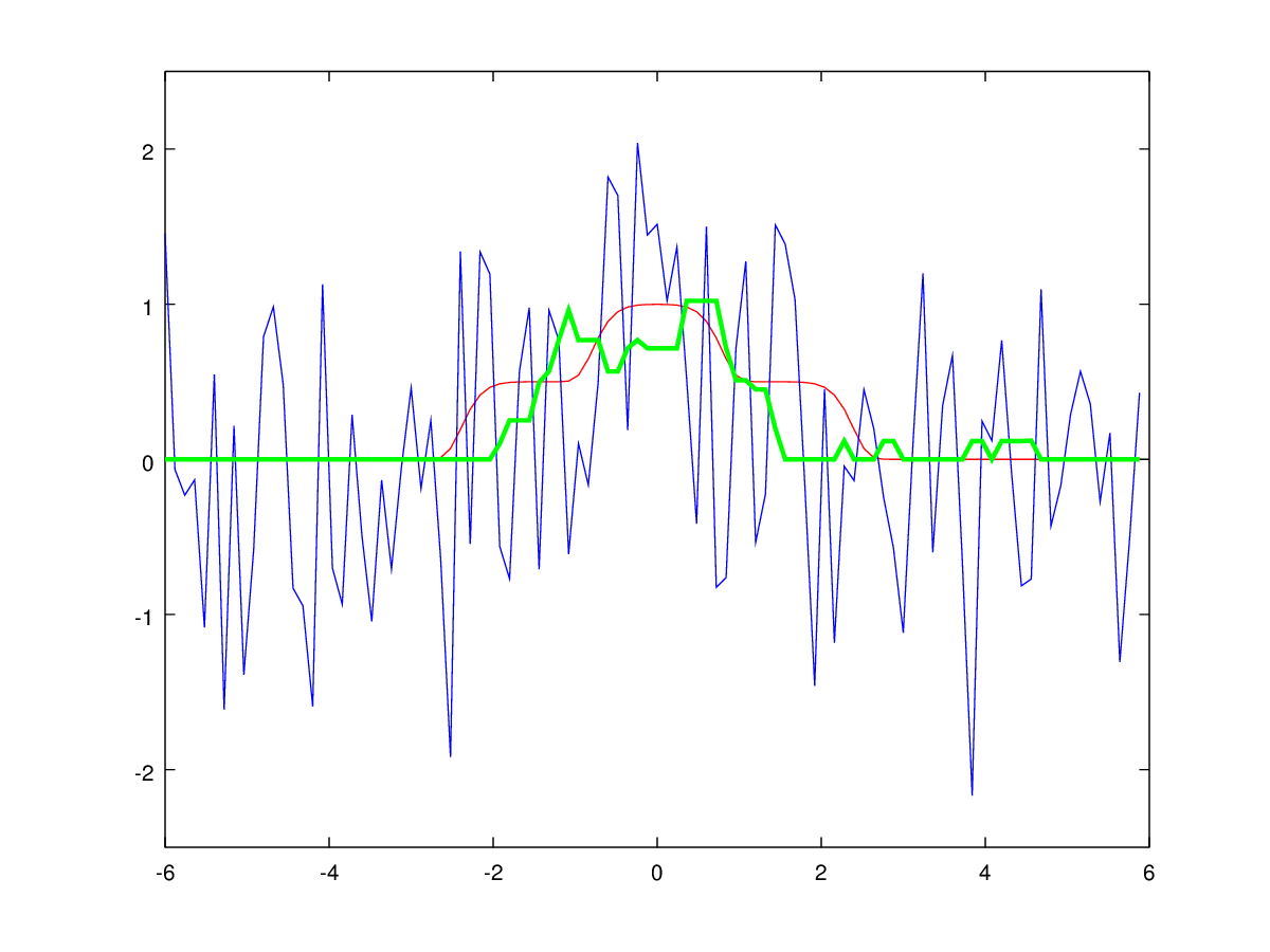
Fig. 7: Median unimodal filtering. The blue color shows the input noisy signal, green - the result of filtering, red - the ideal non-noise signal.
As can be seen, on sufficiently arbitrary data, the dynamic programming method gives a better result than the simplest well-known filters. At the same time, comparing them on model examples in detail is absolutely pointless. The above method is valuable precisely because it is an example of a “suit tailored to measure”: a formalized statement of the problem was laid at the very foundation of the method. In the case under consideration, this was a condition of unimodality. Similarly, linear methods “by measure” to signals that are frequency-separable with noise. Another tool in the kit - what could be better for an engineer?
The problem of offline signal filtering in the case when the expected waveform is known with an accuracy of up to several unknown parameters is reduced to the approximation problem. For example, if it is known that the signal grows linearly over the considered interval, the problem will be reduced to linear regression, and if it can be assumed that the noise is normal, then the correct method will be OLS . But once we faced the task of evaluating the shape of an X-ray microprobe profile (beam), about which only one thing was known a priori: the profile is unimodal, namely, it has exactly one maximum. It turns out that in this case, the best (in the sense, for example, L2 metrics) approach the experimental signal with a function belonging to a known set (a set of unimodal functions). Moreover, with acceptable asymptotics of computational complexity.
===> ===> So, we will talk about the problem of approximation of a certain noisy signal
')
First, for simplicity, it makes sense to consider the same problem for a monotonic function. The description is given for a monotonously non-strictly increasing function, although, of course, for the monotonically decreasing one can do the same.
If we assume that the noise is normally distributed, then the problem will be reduced to minimizing the quadratic functional
There is an alternative solution that does not have these disadvantages, but when using it, the signal scale
Fig. 1: a) Model monotonous signal until the noise increases. b) Model monotonous signal after noise imposing.
It turns out that in the discrete approximation, filtering a normally noisy monotone signal reduces to dynamic programming with two parameters, and using this solution, it is possible to construct a computational circuit of the same complexity for a unimodal case.
You can read about what dynamic programming is here , and how and to which tasks it is used - here .
Monotone filtering by dynamic programming
In the problem under consideration, the dynamic programming table is two-dimensional, its columns i correspond to increasing values of the discrete argument from left to right
The outer loop is conducted along the coordinate i from left to right. For each value
and outside the table, the functionality is considered to be zero.
At the same time, in order not to recalculate each time the minimum at smaller values of j , it is useful to save it during the filling process along with the value of the functional, and since at the end you need to restore the path, it is more convenient to save the value of m at which this minimum was reached:
Then the calculation of the functional itself can be performed in O (1) for each cell:
After the completion of the direct passage, it remains to obtain an approximation in an explicit form. To do this, look for a minimum among the values of the functional for the rightmost column (the column with the highest coordinate i ), and then perform a reverse pass through i , with the index being restored, the value of the filtered signal j * in each column:
Final values
In fig. 2 shows an example of the result of the described algorithm for a monotonous signal.
Fig. 2: Filtering a monotonically increasing signal by dynamic programming. The input noise signal is shown in blue, the result of the algorithm is shown in green, the ideal non-noise signal in red.
On this consideration of the auxiliary monotonous case is completed.
Unimodal signal
Using the result obtained, one can solve the problem of a unimodal signal by filling in 2 tables of the DP: one is filled as for a monotonic function, the second - in the same way, but in the opposite direction. As a result, 2 functionalities are calculated:
Figures 3 and 4 show an example of the original unimodal signal and the result of its processing by the proposed algorithm.
Fig. 3: Noisy unimodal signal.
Fig. 4: Filtering a unimodal signal by dynamic programming. The input noise signal is shown in blue, the result of the algorithm is shown in green, the ideal non-noise signal in red.
Derivative constraint
In case it is known that the signal cannot change faster than some fixed speed
However, in order not to lose in laboriousness, you need to be able to get the minimum value of the functional on the segment [ j - dj , j ] for a constant time.
This can be done using the Van Herk-Gil-Verman algorithm, described, for example, here .
The result of applying the algorithm with the restriction on the derivative
Fig. 5: Filtering a unimodal signal by dynamic programming with a limitation on the rate of change of the signal. The input noise signal is shown in blue, the result of the algorithm is shown in green, the ideal non-noise signal in red.
Exposing black magic
An inquisitive reader may suspect that the same or better results can be achieved in simpler ways. Of course, with certain parameters of the signal and noise, the described technique will be superfluous. In addition, the road you know is shorter. Therefore, for each tricky case a specialist will surely find a favorite method that will give an acceptable result in his hands.
To dispel a sense of possible fraud, in fig. Figures 6 and 7 show examples of signal processing by Gaussian smoothing and median filtering with a zerkalization at zero. Filter parameters were selected in order to obtain an optimal result, but without fanaticism.
Fig. 6: Filtering a unimodal signal with Gaussian smoothing. The blue color shows the input noisy signal, green - the result of filtering, red - the ideal non-noise signal.
Fig. 7: Median unimodal filtering. The blue color shows the input noisy signal, green - the result of filtering, red - the ideal non-noise signal.
As can be seen, on sufficiently arbitrary data, the dynamic programming method gives a better result than the simplest well-known filters. At the same time, comparing them on model examples in detail is absolutely pointless. The above method is valuable precisely because it is an example of a “suit tailored to measure”: a formalized statement of the problem was laid at the very foundation of the method. In the case under consideration, this was a condition of unimodality. Similarly, linear methods “by measure” to signals that are frequency-separable with noise. Another tool in the kit - what could be better for an engineer?
Source: https://habr.com/ru/post/279427/
All Articles