When would you know from what rubbish
poems grow without knowing shame ...

The topic of this post appeared completely unexpectedly, in the process of reading the book “Real-Time C ++”, more specifically in the process of reading section 6.13, which considered the construction of a divider of the measured voltage so that the resulting result was easily (using only the shift operation) scaled. So, at the end of the section on page 121, a formula was given for estimating the error of the resulting quantity, which led me to some confusion. Since this book “can be seen by children” and get an irreparable trauma to the psyche, if they uncritically react to what was written, I created this post to bring a certain order to the understanding of the methodology for estimating measurement errors by young engineers.




To begin with, let us recall the main points, determine the terminology and establish some important facts.
Any measured value always represents only a certain approximation to the measured parameter, and to estimate the degree of deviation of the measured value from the exact value, the concept of the error dX = | X-Xo |, where dX is the absolute error, X is the measured value, Xo is the true value (it is assumed that we know it from somewhere).
Also very important is the relative error qX = dX / Xo (in the same notation), which characterizes the degree of accuracy of the result obtained much better than the absolute (although there are certain problems with Xo = 0 with it). However, the relative error is very often used to indicate the parameters of electronic circuit components in the form of accuracy, for example, resistors - 5% or 1%.
')
It should be borne in mind that we only specify the maximum value of the deviation of the nominal component from its expected value, there are no assumptions about the distribution law of this deviation, it can be a linear distribution, and a triangular, and Gaussian with truncated tails, therefore no assumptions about we do not make the standard deviation and in the future we operate only with the maximum deviation. Such an approach for our case (we are engineers, not trainers) is more correct, it is unlikely that your customers will be satisfied with the scheme that will work in 98% of cases, the scheme we have designed will always work (within acceptable operating conditions, of course).

Since the measured parameters or component parameter values ​​are extremely rarely used in their pure form, and most often they are part of various transfer functions together with other parameters or constants, we need rules for calculating the accuracy characteristics of various expressions of this kind. Once again, we estimate only the maximum error.

We start with the simplest function f (X) = K * X (the scaling function) and obtain the accuracy for the result of this function depending on the accuracy of its members. Assuming the constant K is given exactly, we apply the simplest method of direct calculation qf (X) = | f (X) - f (Xo) | / f (Xo), which leads to the expression q (k * X) = | K * (Xo + dX) - K * Xo | / (K * Xo), or q (K * X) = | K * dX | / (K * Xo) = dX / Xo, hence q (K * X) = qX, which means that the relative error does not change when scaling.

The next important function is taking the inverse value f (X) = 1 / X, for it we get
q (1 / X) = | 1 / (Xo + dX) - 1 / Xo | / (1 / Xo), after transformation we have
q (1 / X) = | -dX / ((Xo + dX) * Xo) | * Xo = | -dX / (Xo + dx) |,
assuming that dX << Xo, we get q (1 / X) ~ dX / Xo = qX, that is, when taking the inverse value, the relative error remains unchanged.

We now consider the sum function f (X, Y) = X + Y. We perform similar calculations and obtain
q (X + Y) = | ((Xo + dX) + (Yo + dY)) - (Xo + Yo) | / (Xo + Yo) = | dX + dY | / (Xo + Yo) = qX * Xo / (Xo + Yo) + qY * Yo / (Xo + Yo). We were convinced that with the addition of two quantities the absolute errors add up, and the relative errors are scaled according to the values ​​of the exact values.
If the relative errors of both quantities coincide, then we get q (X + Y) = qX * (Xo + Yo) / (Xo + Yo) = qX = qY, that is, when adding two quantities with the same relative error, the relative error of the sum will be the same.

An interesting conclusion follows from the results obtained - the relative accuracy of the equivalent resistance of any resistor circuit is equal to the relative accuracy of its components and does not depend on the nominal values ​​and the connection circuit. Indeed, with a series connection, the resistances are added, and we have established the preservation of accuracy when adding, and with a parallel connection, the conductivities (values ​​opposite to the resistance) are added, and we also have established the preservation of accuracy when taking the reverse. The result (at least for me) is somewhat unexpected, but it turns out that way.

For further consideration, we also need the accuracy of the multiplication function of two quantities; we obtain it in the same way.
q (X * Y) = | (Xo + dX) * (Yo + dY) - Xo * Yo | / (Xo * Yo) = | dX * Yo + dY * Xo + dX * dY | / (Xo * Yo) =
= dX / Xo + dY / Yo + dX / Xo * dY / Yo = qX + qY + qX * qY, taking into account qY ~ qY << 1, we finally get q (X * Y) = qX + qY, that is, when multiplying relative errors add up.
Considering division as multiplication by the inverse value, we extend this result to the division q (X / Y) = qX + qY.

Now we are ready to calculate the accuracy of the transfer coefficient of the resistive divider, which is determined by the formula
K (R, r) = r / (R + r). To begin, consider our formula in parts and estimate qK (R, r) = qr + q (R + r) = qr + qR * R / (R + r) + qr * r / (R + r), assuming qr = qR, we get qK (R, r) = 2 * qR.
It is this result that was used in the book indicated at the very beginning of the post, but it is not quite correct, because we believed that the numerator and denominator of the fraction in our function are independent, and this is not so, and there and there the common parameter is used.
Let us clarify the result obtained by resorting to the tried and tested method of obtaining a relative error and get (intermediate calculations are left to the inquisitive reader and so they will surely scold me for the inconvenient writing of formulas, for some reason I don’t have Latex today, and there will be multi-storey expressions) qK (R, r) = (qR + qr) * R / (R + r).
So, we see that the refined error formula shows us that the accuracy of the divider transfer coefficient depends on the division ratio K = r / (R + r) in the form qK (R, r) = 2 * qR * (1 - K), then there is a doubling of the error only for very small transmission coefficients (K << 1), and, for example, with a division ratio of 1/2, the relative error of the coefficient will coincide with the relative error of the resistors, which again is somewhat unexpected. For the nominal values ​​specified in the book, the error will be 2 * 64.9 / (11.8 + 64.9) = 1.7 * qR, which, although close to the first result (2 * qR), is still separated from it.

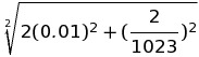
And the last remark - since I repeatedly stressed that we estimate the maximum deviation, the calculation of the rms value can in no way be welcomed and, given that the code at the output of the ADC is described by the formula N = Uin * Kac, you should simply add the relative errors of these quantities, getting qN = qUin + qKatsp = 1.7 * 0.01 + 2/1024 ~ 1.9% <2%, which, however, corresponds to the result indicated in the book.

One more important circumstance should be taken into account - if the error of the transmission coefficient does not depend on the input voltage, then we can’t say about the error of the ADC - it is 2 EMP regardless of the input voltage (in fact, everything is much more complicated, but we accepted for simplicity ), so that the obtained relative measurement error is true only for voltages close to the maximum, and in other cases it will increase.