Linear models: simple regression
Last time we examined in detail the diversity of linear models . Now let's move from theory to practice and build the simplest, but still useful model that you can easily adapt to your tasks. The model will be illustrated with code in R and Python, and in three flavors at once: scikit-learn, statsmodels and Patsy.
Let us be given the initial data in the form of a table with columns x1 , x2 , x3 and y . And we will build a linear model of dependence of y on the factors x , that is, the model will have the following form:
y = b 0 + b 1 x 1 + b 2 x 2 + b 3 x 3 +
where x , y is the initial data, b is the model parameters, ℇ is a random variable.
Since we already have x and y , our task is to calculate the parameters b .
Please note that we have introduced the parameter b 0 , which is also called intercept , since our model line will not necessarily pass through the origin. If the source data is centered, this parameter is not required.
To construct a model, we also need to introduce a parametric assumption regarding ℇ — without this, we cannot choose a solution method. What horrible method we have no right to use, because we risk getting any erroneous result, while we need a “reasonably good” estimation of model parameters. So for simplicity and convenience, we assume that the errors are distributed normally, so we can use the ordinary least squares method.
Please note that all methods for calculating coefficients give the same result. And this is absolutely no coincidence. Due to the normality of errors, the optimized functional (ONC, OLS) turns out to be convex, and therefore has a single minimum, and the desired set of model coefficients will also be unique.
However, even a slight change in the source data, despite the preservation of the form of distributions, will lead to a change in the coefficients. Simply put, although the real life does not change, and the nature of the data also remains unchanged, as a result of the invariable method of calculation you will receive different models, and in fact the model should be the only one. We will talk more about this in the regularization article.
So, we have already built a model ... However, most likely we made a mistake, perhaps even more than one. Since we did not study the data before tackling the model, we received a model of what was not clear. Therefore, let's still look at the data and see what is there.
As you remember, there were 4 columns in the source table: x1 , x2 , x3, and y . And we built a regression dependence of y on all x . Since we cannot immediately cover the entire 4-dimensional hypercube with one glance, we will look at the individual xy plots.
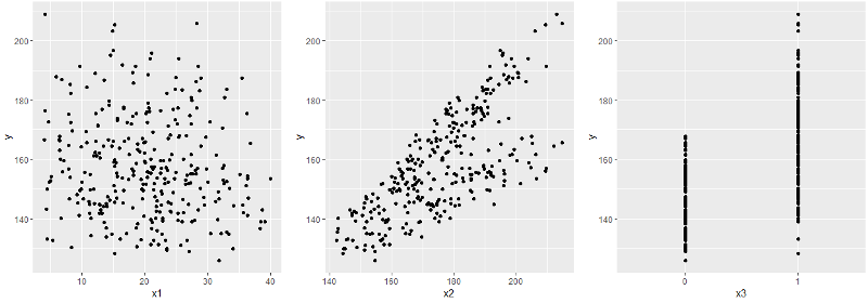
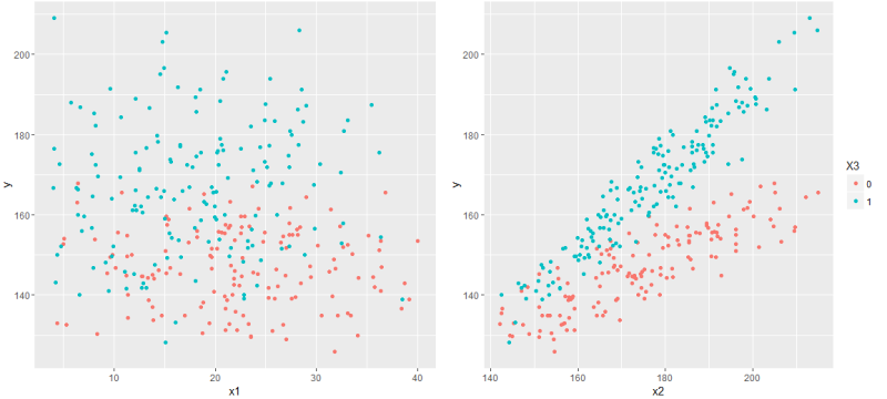
Immediately catches the eye x3 - a binary sign - and with them it is worth being closer. In particular, it makes sense to look at the joint distribution of the remaining x together with x3 .
Now it's time to display the graph corresponding to the constructed model. And here it is worth noting that our linear model is not a line at all, but a hyperplane, so on a two-dimensional graph we will be able to display only a single slice of this model hyperplane. Simply put, to show the model's graph in x1 - y coordinates, you need to fix the values of x2 and x3 , and by changing them, we get an infinite number of graphs - and they will all be graphs of the model (or rather, projection onto the x1 - y plane ).
Since x3 is a binary feature, you can show a separate line for each attribute value, and fix x1 and x2 at the arithmetic average level, that is, draw the graphs y = f (x1 | x2 = E (x2)) and y = f (x2 | x1 = E (x1)), where E is the arithmetic average over all values of x1 and x2, respectively.
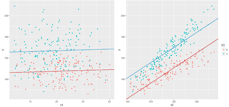
And it immediately catches the eye that the graph y ~ x2 looks somehow wrong. Remembering that the constructed model should predict the expectation y , here we see that the model line does not match the expectation at all: for example, at the beginning of the graph, blue points of real values are below the blue line, and at the end - above, and the red line has on the contrary, although both lines should pass approximately in the middle of a cloud of points.
Looking closer, you can guess that the blue and red lines should even be non-parallel. How to do this in a linear model? Obviously, by building a linear model with y = f (x1, x2, x3) we can get an infinite number of lines of the form y = f (x2 | x1, x3) , that is, fixing two of the three variables. So, in particular, the red line y = f (x2 | x1 = E (x), x3 = 0) and the blue y = f (x2 | x1 = E (x), x3 = 1) are obtained on the right graph. However, all such lines will be parallel.
')
To make the model non-parallel, let’s make it a bit more complicated by adding just one term:
y = b 0 + b 1 x 1 + b 2 x 2 + b 3 x 3 + b 4 x 2 x 3 +
Where it leads? Previously, any line on the graph y ~ x 2 had the same slope, given by the coefficient b 2 . Now, depending on the value of x 3, the line will have a slope b 2 (for x 3 = 0 ) or b 2 + b 4 (for x 3 = 1 ).
And now take a look at the updated schedule.
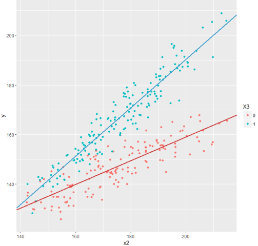
Much better!
This technique - the multiplication of variables - is extremely useful for binary and categorical factors and allows you to actually build several models at once within the same model that reflect the characteristics of different groups of objects studied (men and women, ordinary employees and managers, lovers of classical, rock or pop music ). Particularly interesting models can be obtained when there are several binary and categorical factors in the source data.
At the request of those who wish, I also created a small ipython notebook .
To summarize: we have built a simple, but still very adequate model, which, judging by the graphs, reflects the real data quite well. However, all these “very” and “not bad” are better presented in measurable terms. It also remains unclear how much the built model is resistant to small changes in the initial data or to the structure of these data (in particular, to the interdependence between factors). We will definitely return to these questions.
Simple linear regression
Let us be given the initial data in the form of a table with columns x1 , x2 , x3 and y . And we will build a linear model of dependence of y on the factors x , that is, the model will have the following form:
y = b 0 + b 1 x 1 + b 2 x 2 + b 3 x 3 +
where x , y is the initial data, b is the model parameters, ℇ is a random variable.
Since we already have x and y , our task is to calculate the parameters b .
Please note that we have introduced the parameter b 0 , which is also called intercept , since our model line will not necessarily pass through the origin. If the source data is centered, this parameter is not required.
To construct a model, we also need to introduce a parametric assumption regarding ℇ — without this, we cannot choose a solution method. What horrible method we have no right to use, because we risk getting any erroneous result, while we need a “reasonably good” estimation of model parameters. So for simplicity and convenience, we assume that the errors are distributed normally, so we can use the ordinary least squares method.
R code
# df <- read.csv("http://roman-kh.imtqy.com/files/linear-models/simple1.csv") # # glm intercept, g <- glm("y ~ x1 + x2 + x3", data=df) # coef(g) Python code: common part
import numpy as np import pandas as pd import statsmodels.api as sm import patsy as pt import sklearn.linear_model as lm # df = pd.DataFrame.from_csv("http://roman-kh.imtqy.com/files/linear-models/simple1.csv") # x - (x1, x2, x3) x = df.iloc[:,:-1] # y - y = df.iloc[:,-1] Python code: scikit-learn
# skm = lm.LinearRegression() # skm.fit(x, y) # print skm.intercept_, skm.coef_ Python code: statsmodels
# intercept' x_ = sm.add_constant(x) # (Ordinary Least Squares) smm = sm.OLS(y, x_) # res = smm.fit() # print res.params Python code: statsmodels with formulas
Moving from R to Python, many start with statsmodels, because it has the usual R'ov formulas:
# smm = sm.OLS.from_formula("y ~ x1 + x2 + x3", data=df) # res = smm.fit() # print res.params Python code: Patsy + numpy
Thanks to the Patsy library, you can easily use R-like formulas in any of your programs:
# pt_y, pt_x = pt.dmatrices("y ~ x1 + x2 + x3", df) # numpy' # , LinearRegression scikit-learn # scipy.sparse.linalg.lsqr res = np.linalg.lstsq(pt_x, pt_y) # b = res[0].ravel() print b Please note that all methods for calculating coefficients give the same result. And this is absolutely no coincidence. Due to the normality of errors, the optimized functional (ONC, OLS) turns out to be convex, and therefore has a single minimum, and the desired set of model coefficients will also be unique.
However, even a slight change in the source data, despite the preservation of the form of distributions, will lead to a change in the coefficients. Simply put, although the real life does not change, and the nature of the data also remains unchanged, as a result of the invariable method of calculation you will receive different models, and in fact the model should be the only one. We will talk more about this in the regularization article.
We study the data
So, we have already built a model ... However, most likely we made a mistake, perhaps even more than one. Since we did not study the data before tackling the model, we received a model of what was not clear. Therefore, let's still look at the data and see what is there.
As you remember, there were 4 columns in the source table: x1 , x2 , x3, and y . And we built a regression dependence of y on all x . Since we cannot immediately cover the entire 4-dimensional hypercube with one glance, we will look at the individual xy plots.
Immediately catches the eye x3 - a binary sign - and with them it is worth being closer. In particular, it makes sense to look at the joint distribution of the remaining x together with x3 .
Now it's time to display the graph corresponding to the constructed model. And here it is worth noting that our linear model is not a line at all, but a hyperplane, so on a two-dimensional graph we will be able to display only a single slice of this model hyperplane. Simply put, to show the model's graph in x1 - y coordinates, you need to fix the values of x2 and x3 , and by changing them, we get an infinite number of graphs - and they will all be graphs of the model (or rather, projection onto the x1 - y plane ).
Since x3 is a binary feature, you can show a separate line for each attribute value, and fix x1 and x2 at the arithmetic average level, that is, draw the graphs y = f (x1 | x2 = E (x2)) and y = f (x2 | x1 = E (x1)), where E is the arithmetic average over all values of x1 and x2, respectively.
And it immediately catches the eye that the graph y ~ x2 looks somehow wrong. Remembering that the constructed model should predict the expectation y , here we see that the model line does not match the expectation at all: for example, at the beginning of the graph, blue points of real values are below the blue line, and at the end - above, and the red line has on the contrary, although both lines should pass approximately in the middle of a cloud of points.
Looking closer, you can guess that the blue and red lines should even be non-parallel. How to do this in a linear model? Obviously, by building a linear model with y = f (x1, x2, x3) we can get an infinite number of lines of the form y = f (x2 | x1, x3) , that is, fixing two of the three variables. So, in particular, the red line y = f (x2 | x1 = E (x), x3 = 0) and the blue y = f (x2 | x1 = E (x), x3 = 1) are obtained on the right graph. However, all such lines will be parallel.
')
Non-parallel linear model
To make the model non-parallel, let’s make it a bit more complicated by adding just one term:
y = b 0 + b 1 x 1 + b 2 x 2 + b 3 x 3 + b 4 x 2 x 3 +
Where it leads? Previously, any line on the graph y ~ x 2 had the same slope, given by the coefficient b 2 . Now, depending on the value of x 3, the line will have a slope b 2 (for x 3 = 0 ) or b 2 + b 4 (for x 3 = 1 ).
R code
# df <- read.csv("http://roman-kh.imtqy.com/files/linear-models/simple1.csv") # # glm intercept, g <- glm("y ~ x1 + x2 + x3 + x2*x3", data=df) # coef(g) Python code: common part
import numpy as np import pandas as pd import statsmodels.api as sm import patsy as pt import sklearn.linear_model as lm # df = pd.DataFrame.from_csv("http://roman-kh.imtqy.com/files/linear-models/simple1.csv") # x - (x1, x2, x3) x = df.iloc[:,:-1] # y - y = df.iloc[:,-1] Python code: scikit-learn
# x["x4"] = x["x2"] * x["x3"] # skm = lm.LinearRegression() # skm.fit(x, y) # print skm.intercept_, skm.coef_ Python code: statsmodels
# x["x4"] = x["x2"] * x["x3"] # intercept' x_ = sm.add_constant(x) # (Ordinary Least Squares) smm = sm.OLS(y, x_) # res = smm.fit() # print res.params Python code: statsmodels with formulas
Moving from R to Python, many start with statsmodels, because it has the usual R'ov formulas:
# smm = sm.OLS.from_formula("y ~ x1 + x2 + x3 + x2*x3", data=df) # res = smm.fit() # print res.params Python code: Patsy + numpy
Thanks to the Patsy library, you can easily use R-like formulas in any of your programs:
# pt_y, pt_x = pt.dmatrices("y ~ x1 + x2 + x3 + x2*x3", df) # numpy' # , LinearRegression scikit-learn # scipy.sparse.linalg.lsqr res = np.linalg.lstsq(pt_x, pt_y) # b = res[0].ravel() print b And now take a look at the updated schedule.
Much better!
This technique - the multiplication of variables - is extremely useful for binary and categorical factors and allows you to actually build several models at once within the same model that reflect the characteristics of different groups of objects studied (men and women, ordinary employees and managers, lovers of classical, rock or pop music ). Particularly interesting models can be obtained when there are several binary and categorical factors in the source data.
At the request of those who wish, I also created a small ipython notebook .
To summarize: we have built a simple, but still very adequate model, which, judging by the graphs, reflects the real data quite well. However, all these “very” and “not bad” are better presented in measurable terms. It also remains unclear how much the built model is resistant to small changes in the initial data or to the structure of these data (in particular, to the interdependence between factors). We will definitely return to these questions.
Source: https://habr.com/ru/post/279117/
All Articles