Parametric identification of a linear dynamic system

Introduction

Dear readers. Currently, the processes of identification of dynamic systems are given much attention. Many dissertations, diplomas and scientific publications have been written on this topic. In various literature, a lot of things have been written about identification, various models and methods are given. But all this for the average man becomes not immediately clear. In this article I will try to explain how to solve a parametric identification problem, when a technical system (object) is described by a system of differential equations, using the OLS method.

A bit of theory

First you need to understand what a dynamic system . Speaking as simply as possible, this is a system whose parameters change over time. Read more here . Virtually any dynamic system can be described by a differential equation of some order, for example:

${{dx_1 \ over dt} = ax_1 + bx_2} \\ {dx_2 \ over dt} = cx_1 + dx_2}.$

This system of differential equations is characterized by its parameters. In our case, these are a , b , c, and d . They can be both static and dynamic .
')

What do these factors mean?

Applied to real physical dynamic systems, these coefficients of a differential equation have a specific physical reference. For example, in the system of orientation and stabilization of a spacecraft, these coefficients may play a different role: the coefficient of static stability of the spacecraft , the coefficient of efficiency of the onboard control, the coefficient of ability to change the trajectory, etc. Read more here .

So the problem of parametric identification is the definition of these ~~coefficients of the~~ parameters a , b , c and d .

The task of observation and measurement

It should be noted that to solve the problem of parametric identification, it is necessary to obtain “measurements” of one (or all) phase coordinates (in our case, this is x ₁ and (or) x ₂ ).

In order for the system to be identifiable, it must be observable. That is, the rank of the observability matrix must be equal to the order of the system. Read more about observability here .

Observation of the processes occurring in the object, is as follows:

$y = Hx + \ xi (t).$

Where:

y is the vector of observed parameters;
H is the coupling matrix of the state parameters and the observed parameters;

$\ xi (t)$ - interference component (it hides all the errors of observation);

More about vectors and matrices

The dynamic system that we described above can be represented in a vector-matrix form:

${dx \ over dt} = Ax + Bu + \ varepsilon (t)$

Where:

x is the state vector of the dynamic system. In general, it has infinite dimension. But when we deal with a specific model, we are already talking not about the “state vector” but about the “vector of phase coordinates”. In our example, it has two components.
$x = \ begin {pmatrix} x_1 \\ x_2 \ end {pmatrix}$
A - transition matrix. It contains the very factors that we would like to find.
$A = \ begin {pmatrix} a & amp; b \\ c & amp; d \ end {pmatrix}$
u - control action. In our example, it is equal to 0. That is, our object is not controlled. Please note that this is just an example, which has nothing to do with any real-life system.
B - control matrix.

$\ varepsilon (t)$ - jamming component.

Measuring the processes occurring in the object is described as follows:

${{z} = y + n (t)} \\ {z} = n_1 (t) y + n_2 (t)}.$

As we see, the measurement error can be both additive (in the first case) and multiplicative (in the second)

Identification task

Consider the solution of the problem of parametric identification in the case when one coefficient is not known. Let us turn to a specific example. Let the following system be given:

${{dx_1 \ over dt} = ax_1 + x_2} \\ {dx_2 \ over dt} = 0.0225x_1-0.3x_2} \\ {x_1 (0) = 20 \ x_2 (0) = 20}$

It can be seen that the parameters are b = 1 , c = 0.0225 and d = -0.3 . The parameter a is unknown to us. Let's try to estimate it using the method of least squares.

The task is as follows: according to the available sampling data of observations of the output signals with the sampling interval Δt, it is required to estimate the parameter values that ensure the minimum value of the residual functional between the model and actual data.

$J = (y-y_m) ^ T (y-y_m) = e ^ Te = \ sum \ limits_ {j = 1} ^ {N} e_j ^ 2 \ longrightarrow \ min$

Where $e_j = y_i-y_m_i$ - discrepancy, defined as the difference between the output of the object under study and the reaction calculated by the mathematical model of the object.

The discrepancy consists of inaccuracies in the structure of the model, measurement errors and unaccounted interactions of the environment and the object. However, regardless of the nature of the errors, the least squares method minimizes the sum of the quadratic residual for discrete values. In principle, the MNC does not require any a priori information about the interference. But in order for the resulting estimates to have desirable properties, we will assume that the interference is a random process such as white noise.

Evaluation $a ^ *$ the least squares method that minimizes the J criterion is found from the condition for the existence of a minimum of the functional:

$J = \ min \ limits_ {a} J = J | _ {a = a ^ *}$

An important property of OLS estimates is the existence of only one local minimum, which coincides with the global one. Therefore, the assessment $a ^ *$ is the only one. Its value is determined from the condition of the extremum of the functional J :

${{\ partial J \ over \ partial a} | _ {a = a ^ *} = 2 (y-y_m) (y-y_m) ^ {\ prime} = 0$

That is necessary from the functional $J = (y-y_m) ^ 2$ take the derivative with respect to a and equate it to zero.

I pay attention that $y$ - this is the "measured" values of the phase coordinates $x_1$ and (or) $x_2$ , but $y_m$ - these are phase coordinates $x_1$ and (or) $x_2$ calculated by the mathematical model of the object. But after all, in the object model, represented as a system of differential equations, $x_1$ and $x_2$ not expressed explicitly. In order to get rid of this ~~madness,~~ it is necessary to solve this system of differential equations with given initial conditions.

You can solve both "manually" and using any software. The solution in MatLab will be shown below. The result should be a system of algebraic equations for each point in time. $t_i$ :

$Sa_i ^ * = y_i$

Then substituting instead $y$ the values of the "measured" phase coordinates, find the parameter estimate $a_i ^ *$ for each point in time $t_i$ .

Where to get these “measured” values of phase coordinates?

In general, these values are taken from the experiment. But since we did not conduct any experiment, we take these values from the numerical solution of our system of differential equations using the Runge – Kutt method of 4–5 orders of magnitude. Choose a parameter $a = -0.7$

The solution is found by the built-in functions of the MatLab package. Read more here . The solution to this method is shown below.

MatLab code

function F = diffurafun (t, x)
F = [- 0.7 * x (1) + x (2); 0.0225 * x (1) -0.3 * x (2)];
end
% ================================================ ==============%
% formation of the vector of initial conditions
X0 = [20; 20];
% formation of the integration interval
interval = [0 50];
% access function ode 45
[T, X] = ode45 (@ diffurafun, interval, X0);
% output solution graph
figure; plot (T, X (:, 1), 'r -', T, X (:, 2), 'b--'); % output graph
legend ('Parameter x1', 'Parameter x2');
grid on;

Schedule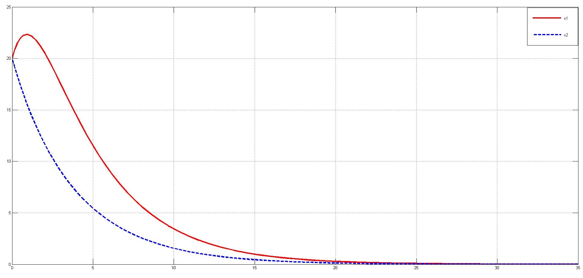

In this graph, the red solid line indicates the phase coordinate $x_1$ , and the blue dotted line indicates the phase coordinate $x_2$

Below is the MatLab code and graph.

MatLab Code

% dx / dt = A * x - linear dynamic system without control and interference
% for the beginning we need to solve analytically this CDS
% denote the type of variables
syms x (t) y (t) a
% solve the system for the given initial conditions
S = dsolve (diff (x) == a * x + 1 * y, 'x (0) = 20', diff (y) == 0.0225 * x - 0.3 * y, 'y (0) = 20') ;
% choose the solution of the first phase coordinate, since it is in its equation
% contains the required parameter a
x (t) = Sx;
% we find the partial derivative of the first equation in the parameter a (in
% accordance with the method of OLS)
f = diff (x (t), 'a');
% now slightly simplify the resulting expression
S1 = simplify (f);
% set the variable t array of values T
t = t;
% we find the expression containing the parameter a for each point in time
SS = eval (S1);
% is now in a loop, substituting the value "measured" in each expression
% of the first phase coordinate, we define the parameter a for each moment
% of time T. We take the values of the “measured” phase coordinate from the solution of the SDE
% by the method of Runge-Kutta 4th order
for i = 2: 81
SSS (i) = solve (SS (i) == X (i, 1), a);
end
ist = zeros (length (T), 1);
ist (1: length (T)) = - 0.7;
figure; plot (T, SSS, 'b -', T, ist, 'r-');
legend ('parameter estimate a', 'true value');
grid on;

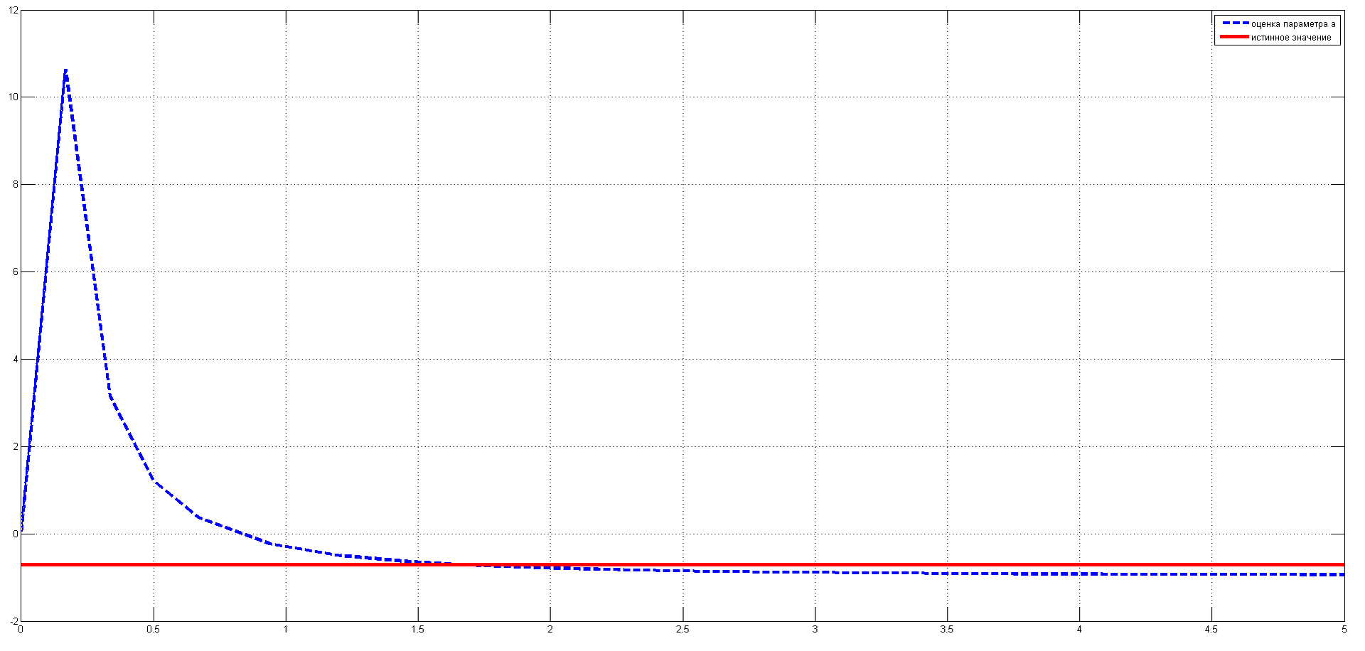
The blue dotted line in the graph indicates the parameter estimate. $a ^ *$ , and the red solid line indicates directly the “true” value of the model parameter $a = -0.7$ . We see that the process stabilizes in about 3.5 seconds. Small discrepancy of parameter estimation $a ^ *$ and the “true” value is caused by errors in solving the system of differential equations by the Runge-Kutt method.

Source: https://habr.com/ru/post/279025/

All Articles

Parametric identification of a linear dynamic system

Introduction

A bit of theory

The task of observation and measurement

Identification task

More articles: