Grid implementation for working with large tables. Part 1

A table (grid) with a vertical scroll bar is the most common user interface element for working with data from a relational database. However, the difficulties are encountered that are encountered when the table contains so many entries that the tactics of their complete reading and storage in the operational memory becomes unreasonable.

Some applications on large tables are not calculated and “freeze” when you try to open a table with millions of records for viewing / editing. Others refuse to use the vertical scroll bar in favor of paging or offer the user only the illusion that you can quickly jump to the desired (at least to the latest) entry with the scroll bar.


')
We will talk about one of the possible methods for implementing a tabular control that has the properties of Log (N) -fast 1) initial display 2) scrolling over the entire range of records 3) switching to a record with a given unique key. All this - with two restrictions: 1) records can be sorted only by the indexed set of fields and 2) the database collation rules should be known to the algorithm.

The principles outlined in the article were implemented by the author in a project with his participation in the Java language.

The basic principle

The two key functionalities of the table control (grid) are

1. scroll - Displays entries corresponding to the position of the scroll bar,
2. Jump to the record specified by the combination of key fields.

First, we consider the simplest approaches to their implementation and show why they are unsuitable in the case of a large number of records.

The most straightforward approach is to read all the records into the RAM (or at least their primary keys), after which the scrolling is done by selecting the array segment, and the positioning is done by searching the record in the array. But with a large number of records, firstly, the process of initial loading of the array takes too much time and, as a result, the display of the grid on the screen is delayed, and secondly, these tables start to take up memory, which reduces the overall speed.

Another approach is to “shift” the calculations to the DBMS: the selection of records for display in the scrolling window is carried out using the constructions like select ... limit ... offset ... , positioning - reduce to select ... and count (*). However, both offset and count (*) are associated with enumerating the records inside the server, they generally have O (N) execution speed, and therefore are inefficient with a large number of records. Calling them often leads to an overload of the database server.

So, we need to implement a system that would not require the full downloading of data into memory and at the same time would not overload the server with inefficiently running queries. To do this, we understand which queries are effective and which are not.

Provided that an index is built across the k field, the following queries are fast (they use the index lookup and are executed during Log (N)):

1. Query A. Find the first and last entry in the dataset:
   

   select ... order by k [desc] limit 1 

2. Request B. Find the h of the first entries with a key greater than or equal to the given value of K:

    select ... order by k where k >= K limit h 

A remarkable property of query B is that, as a parameter, it does not have to substitute the key for an existing record in the database: it equally quickly finds both the record by its primary key and the record closest to the specified key. We will actively use this.

The following queries are not fast:

1. Query C Calculate the total number of records in the dataset:
   

    select count(*) ... 

2. Request D. Count the number of records preceding the record with a key greater than or equal to this one:
   

    select count(*) ... where key < K 

Requests B and D can be generalized to the case of sorting by a set of several fields order by k1, k2, k3 ... provided that a composite index is built on these fields. The condition k> = K should be generalized to a logical condition for comparing several values ​​in the lexicographical order :

 where k1 >= K1 and (k1 > K1 or (k2 >= K_2 and (k2 > K2 or ...))) 

The basic principle is that in procedures that require a quick response for the user, only quick queries to the database are dispensed with.

"Guessing" the dependence of the primary key on the record number

For the time being, imagine that the primary key of our table has only one integer field (hereinafter, we will remove this restriction).

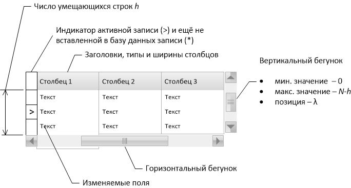
Let each position of the scroll bar correspond to an integer from 0 to where - total number of records in the table, - the number of lines that fit on one page in the grid. If the scroll bar is set to then this means that when drawing the grid you should skip first entries in the table and then output records. This is exactly what the keywords offset and limit in PostgreSQL are responsible for, and with a large number of records we cannot use them. But if in some “magic” way we could be able to calculate the function and its inverse function that connects the primary key and the number of records with a key smaller than this one, then using query B , substituting the value , we could quickly get a set of records to display to the user. The task of moving to the desired record would be solved in the following way: since the primary key is known in advance, it can immediately be used as a parameter of quick query B , and the scroll bar should be set to . The task would be solved!

(Note that the query D , called with the parameter k, just returns the value but 1) it is slow and 2) we need to be able to calculate how , and the opposite to her.)

Naturally, the function completely determined by the data in the table, therefore, in order to accurately restore the interdependence of key values ​​and record numbers, it is necessary to read all the keys from the database into main memory through one : for a correct response of query B at intermediate points, we can assume that (recall the remarkable property of query B ). This is better than remembering all keys in a row, but still not good enough, because it requires O (N) time and RAM to initially display the table. Fortunately, you can get by with a much smaller value of exactly known points for the function and in order to understand this, we will need a small combinatorial analysis of possible values .

Let us execute the query

 select min(k), max(k), count(*) from foo 

and got the results: 0, 60, 7. That is, we now know that there are only 7 records in our table (and this means the maximum value equal to 6), the first of the entries has the key 0, and the last - the key 60. With one such query, we actually learned the values in three points : , and . And that's not all, because from the definition itself follows that:

1. monotonously grows
2. while increasing per unit increases by one or not increases, so the function graph except point , entirely in parallelogram , , , ,
3. total number of possible functions equal to the number of distribution methods records by key values ​​(the positions of the first and last entries are fixed), i.e.
   
   
   
   
   
4. number of possible functions which are at take on meaning , is determined by the product of the number of combinations of records with a key less than and greater or equal :
   
   
   
   
   

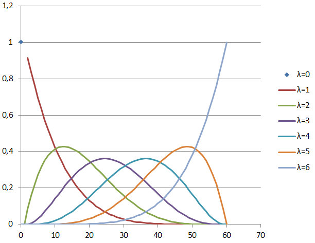
Thus, if each of the possible options is considered equiprobable, then the probability that for a given value there is exactly records with a key strictly smaller given by the relationship known as the hypergeometric distribution . For , the picture looks like this:



The properties of the hypergeometric distribution are well known. When is always and in the segment average value linearly dependent on k:


Value variance has the shape of an inverted parabola with zeros at the edges of the segment and maximum in the middle
(It can be roughly considered that the average error is less than .)

The calculation of the values ​​for the above formulas for , shows such a picture for possible minimum and maximum (red lines), average (blue line) values , as well as the limits of the standard deviation (gray area):



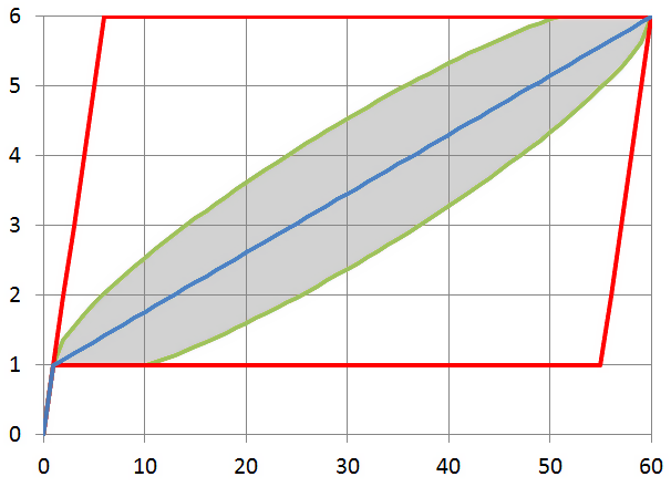
So, the polyline, built between the points , and is a statistically valid approximation for calculating a function and reverse , and this approximation allows us to quite accurately “guess” the values ​​of a function, even if all we know about it is its values ​​at three points, obtained with a single query. In fact, we, for "guessing", perform the first iteration of the interpolation search algorithm, only by accurately determining the boundary values.

If now for some , new exact value will be known we can add a couple to the interpolation table and using piecewise interpolation to obtain a refined calculation of the value to solve the scrolling problem, and applying the inverse piecewise interpolation, calculate the refined value in solving the problem of positioning. With each accumulated point, the range of possible discrepancies will be narrowed, and we will get an increasingly accurate picture for the function .

If there are several key fields and data types are not INT

In practice, the case is not limited to a single integer field for sorting the data set. First, the data type can be different: string, date, and so on. Secondly, there can be several sortable fields. This difficulty is eliminated if we are able to calculate

1. numbering function which translates a set of field values ​​of arbitrary types into a natural number,
2. inverse function which takes the natural number back to the set of field values, .

The numbering function must have the property that if the set less set in the sense of a lexicographic order, then it should be .

Speaking the language of mathematics, bijection must establish an order isomorphism between the set of possible values ​​of sets of fields and the set of natural numbers. Note: in order for the search task to be suitable was mathematically solvable, it is important that the sets of possible field values were finite. For example, it is impossible to construct an order isomorphism between the set of all lexicographically ordered pairs of natural (pairs of real) numbers and the set of natural (real) numbers. Of course, the set of all possible values ​​of any machine data type is finite, although very large.

To represent values standard 32-bit and 64-bit integer types are not suitable: so that one can count only various possible 10-byte strings, a 64-bit (8-byte) integer is not enough. In our implementation, we used the java.math.BigInteger class, which is capable of representing integers of arbitrary size. At the same time, the amount of RAM occupied by the value , approximately equal to the volume occupied by the set of values .

With a reversible numbering function and reversible interpolator function ,

• scrolling the grid is reduced to calculating the values ​​of key fields where - the position of the vertical scroll bar, after which a quick query to the database finds first records, greater or equal ,
• positioning is reduced to reading the first records from the database by the previously known values , and to calculate the position of the scroll bar .

Procedure Interaction Scheme

At this stage, we can escape from mathematics and deal with the algorithmic part itself. The general scheme of interaction between the procedures of the system is shown in the figure below. The “approximate UML Activity” notation is used, with a solid arrow showing the sequence of procedures, and a dotted arrow - an asynchronous call in a separate execution thread:



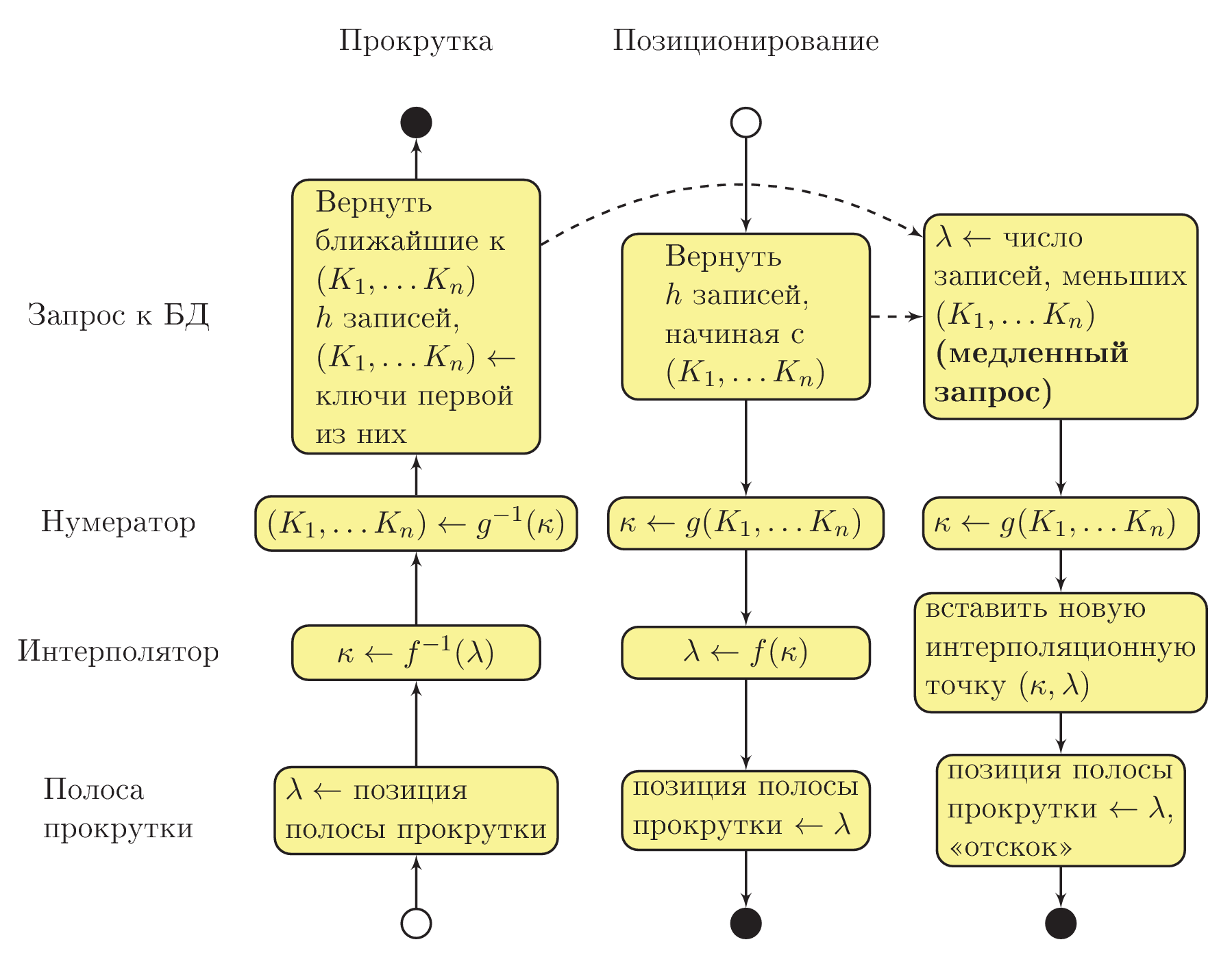
Assume that the user has changed the position of the slider for the vertical scroll bar (see the lower left corner of the chart). Interpolator calculates the value of the number of combinations of the values ​​of key fields ( ) with type BigInteger. Based on this value, the numerator restores the combination of key fields. .

Here it is important to understand that at this stage in the fields there will not necessarily be values ​​that are actually present in the database: there will only be approximations. In string fields, for example, there will be a meaningless set of characters. However, due to the remarkable property of query B , the output from the database strings with keys greater than or equal to the set , will be approximately the right result for a given position of the scroll bar.

If the user released the scroll bar and did not touch it for some time, asynchronously (in a separate execution thread), query D is run, which determines the sequence number of the record, and hence the exact position of the scroll bar, which corresponds to what is displayed to the user. When the query is completed, an interpolation table will be filled up based on the data received. If at this moment the user has not started to scroll the table again, the vertical slider will “bounce” to a new, refined position.

When you go to the record, the sequence of procedure calls is reversed. Since the values ​​of the key fields are already known, for the user, the request B immediately extracts data from the database. The numerator calculates , and then the interpolator determines the approximate position of the scrollbar as . In parallel, in the asynchronous execution flow, a lookup is performed, according to the results of which a new point is added to the interpolation table. After a second or two, the scroll bar will “bounce” to a new, specified position.

The more the user will “wander” according to the vertical slider, the more points will be collected in the interpolation table and the less will be the “bounces”. Practice shows that only 4-5 successful points in the interpolation table are enough for the “bounces” to become very small.

An instance of an interpolator class must hold intermediate points of a monotonously growing function between a set of 32-bit integers (record numbers in a table) and a set of objects of type BigInteger (sequence numbers of combinations of values ​​of key fields).

Immediately after the grid is initialized, you need to request the total number of records in the table in a separate execution flow in order to get the correct value. . Until this value is obtained using a query running in a parallel thread, you can use some default value (for example, 1000) - this will not affect the correctness of the work.

The interpolator must be able to calculate the value of one or the other in a fast way by the number of interpolation points. However, we note that more often it is necessary to calculate the value of the sequence number of a combination by the number of the record: such calculations are performed many times per second during the user scrolling the grid. Therefore, the basis of the implementation of the interpolator module is convenient to take a dictionary based on a binary tree, the keys of which are the record numbers, and the values ​​are the sequence numbers of the combinations (the TreeMap <Integer, BigInteger> class in the Java language).

It is clear that by a given number such a dictionary for logarithmic time finds two points ( ) between which builds direct interpolation of the function . But the fact that grows monotonously, allows for a reverse calculation in a fast time. Indeed: if given a combination number , , search for piecewise segment in which lies can be produced in the dictionary by the dichotomy method. Having found the desired segment, we perform the inverse interpolation and find the number corresponding to .

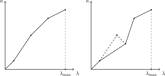
When replenishing the dictionary with interpolation points, it is necessary to ensure that the interpolated function remains monotonous. Since other users can delete and add entries to the table being viewed, the relevance of interpolation points known to the dictionary may be lost, and the newly added point may break the monotony. Therefore, the method of adding a new interpolation point should verify that the “point to the left” of the newly added one corresponds to a smaller one, and to the “point to the right” is a larger value. If it turns out that this is not the case, one should proceed from the assumption that the last point added corresponds to the current state of affairs, and some of the old points have lost their relevance. In relation to the newly added point, all points on the left that contain the larger value and all points on the right that contain the smaller value should be deleted. The process of "cutting out the outgoing point" is shown in the figure:



Also, the interpolator must contain a mechanism in order to save memory protecting the dictionary from overflowing with unnecessary points, and discarding the least significant of them (as we remember, it does not make sense to store all the points in a row - it is enough only through one).

Conclusion to the first part

So, we figured out how our system works in general: its main parts are the interpolator and the numerator , and we also fully discussed the implementation of the interpolator. To complete the solution of the problem, it is now necessary to implement a numerator - a bijection , associating sets of key field values, possibly consisting of dates, strings, sorted using Unicode collation rules, etc., with numbers growing in the same order.

This is the second part of the article .

I am also preparing a scientific publication, and you can also familiarize yourself with the preprint of the scientific version of this article at arxiv.org .