A couple of hours from the life of a mathematician programmer or read Wikipedia

To begin with, I quote rocknrollnerd as an epigraph:

- Hello, my name is% username%, and secretly open the amount of sigma notation on a piece of paper to understand what is happening there.
- Hi% username%!

So, as I said in my last article, I have students who are afraid of mathematics in panic , but as a hobby, they pick at a soldering iron and now they want to assemble a segway cart. They collected something, but she does not want to keep balance. They thought to use the PID controller , but they just did not manage to pick up the coefficients to make it work well. They came to me for advice. And I have never been a boom boom at all in control theory, I have never come close. But once on Habré, I saw an article that said that the linear-quadratic regulator helped the author, but did not help.

If I still imagine the FID on my fingers ( here’s my article , which I transferred from some kind of fright to hypertext), then I didn’t even hear about other control methods. So, my task is to imagine (and explain to students, and at the same time to you) what a linear-quadratic regulator is. So far, there will be no work with iron, I’ll just show you how I work with literature, because this is exactly the lion’s share of my work.
')
Since exhibitionism about my work has gone, here is my workplace (clickable):

Sources used

So, the first thing I do is go to Wikipedia . Russian Wikipedia is cruel and merciless, therefore we read only English text. He, too, is disgusting, but still not so much. So, we read. Of all the introductory bricks of the text, only one phrase interested me:

Operating system of the system. The problem is that the system is called the LQ problem.

Translated into Russian, they say that they model a certain dynamic system with differential equations (oh, horror), and they choose control directly, minimizing some kind of quadratic function (oh, I feel the approximation of least squares). So good. We are trying to read further:

Finite-horizon, continuous-time LQR,
[a series of horrible formulas]

We skip it, well, it’s like reading into a swamp, besides, it’s obviously disgusting to use hands to count continuous functions.

Infinite-horizon, continuous-time LQR,
[a series of even more awful formulas]

Hour of the hour is not easier, more and improper integrals have gone, we skip, all of a sudden we will find something interesting.

Finite-horizon, discrete-time LQR

Oh, I love it. We have a discrete system, we look at its state at certain intervals (some intervals in the first reading are always equal to one second) of time. Derivatives of the equation are gone, because they can now be approximated as (x_ {k + 1} -x_ {l}) / 1 second. Now it would be nice to understand what x_k is.

One dimensional example

Feynman wrote exactly how he read all the equations, that he accounted for:

Actually, there was a certain amount. I had a scheme, which I am today
something that i'm trying to understand: i keep making up examples. For instance, the mathematicians would come in with a terrific theorem, and they're all excited. I construct something which fits all the conditions. You know, you have a set (one ball) - disjoint (two balls). There are more conditions on. Finally, I’m saying, “False!”

Well, what are we, steeper than Feynman? Personally, I do not. So let's do it. There is a car traveling with a certain initial speed. The task to accelerate it to a certain final speed, while the only thing we can influence is the gas pedal, that is, to accelerate the car.

Let's imagine a car is perfect and moves according to this law:


x_k is the speed of the car per second k, u_k is the position of the gas pedal, which we want, we can interpret it as acceleration per second k. So, we start with a certain speed x_0, and then we perform here such numerical integration (into which words we went). Note that I do not add m / s and m / s ^ 2, u_k is multiplied by one second between the measurements. By default, I have all the coefficients either zero or one.

So, in order to understand what is going on, I write such code here (I write a lot of one-time code that I throw out immediately after writing). I am listing here just in case, as usual, I use OpenNL to solve large sparse linear systems of equations.



So let's figure out what I'm doing. For a start, I say N = 60, I take 60 seconds to everything. Then I say that the final speed should be 2.3 meters per second, and the initial half meter per second, it is set from the bald. I will have 60 * 2 variable variables - 60 values ​​of speed and 60 values ​​of acceleration (strictly speaking, acceleration should be 59, but it's easier for me to say that there are 60 of them, and the latter should be strictly zero).

So I have 2 * N variables (N = 60), even variables (I start counting from scratch, like any normal programmer) is speed, and odd ones are acceleration. I set the initial and final speed with these lines:
In fact, I said that I want the initial speed to be x0 (.5m / s), and the final speed - xN (2.3m / s).

  nlBegin(NL_ROW); // x0 = x0 nlCoefficient(0, 1); nlRightHandSide(x0); nlScaleRow(hard_penalty); nlEnd(NL_ROW); nlBegin(NL_ROW); // xN = xN nlCoefficient((N-1)*2, 1); nlRightHandSide(xN); nlScaleRow(hard_penalty); nlEnd(NL_ROW); 

We know that x {i + 1} = xi + ui, so let's add N-1 such equation to our system:

  for (int i=0; i<N-1; i++) { nlBegin(NL_ROW); // x{i+1} = xi + ui nlCoefficient((i+1)*2 , -1); nlCoefficient((i )*2 , 1); nlCoefficient((i )*2+1, 1); nlScaleRow(hard_penalty); nlEnd(NL_ROW); } 

So, we have added all the hard constraints to the system, but what exactly, in fact, can we want to optimize? Let's just start by saying that we want x_i to reach the final speed xN as soon as possible:

  for (int i=0; i<N; i++) { nlBegin(NL_ROW); // xi = xN, soft nlCoefficient(i*2, 1); nlRightHandSide(xN); nlEnd(NL_ROW); } 

Well, our system is ready, strict rules for the transition between states are given, the quadratic function of the system quality too, let's shake the box and see what the smallest squares give us x_i, u_i as a solution (the red line is speed, green is acceleration):



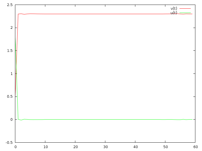
Oookey, we really sped up from half a meter per second to two meters a decimal point of three per second, but our system produced a lot of acceleration (which is logical, because we demanded to converge as soon as possible).

And let's change ( here’s a commit ) the objective function, instead of the fastest convergence, ask for the least possible acceleration:

  for (int i=0; i<N; i++) { nlBegin(NL_ROW); // ui = 0, soft nlCoefficient(i*2+1, 1); nlEnd(NL_ROW); }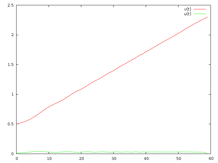 

Hmm, now the car accelerates two meters per second for a full minute. Ok, let's take a quick convergence to the final speed, and try a small acceleration ( commit here )?

  for (int i=0; i<N; i++) { nlBegin(NL_ROW); // ui = 0, soft nlCoefficient(i*2+1, 1); nlEnd(NL_ROW); nlBegin(NL_ROW); // xi = xN, soft nlCoefficient(i*2, 1); nlRightHandSide(xN); nlEnd(NL_ROW); } 

Aha, super, now it becomes beautiful:



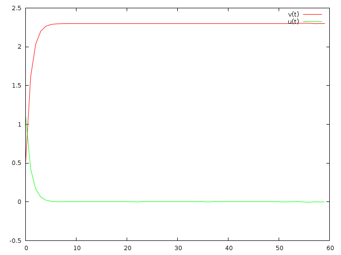
So, fast convergence and limitation of the control value are competing goals, of course. Pay attention, at the moment I stopped at the first line of a Wikipedia paragraph, scary formulas go further, I do not understand them. Often, reading articles is reduced to searching for keywords and the complete conclusion of all the results, using the mathematical device that I personally own.

So what do we have at the moment? The fact that having the initial state of the system + having the final state of the system + number of seconds, we can find the perfect control u_i. This is good, only applies to segway. Damn, how are they doing something? So, read the following text in Wikipedia:

with a performance index defined as



minimizing the performance index is given by



where [AAA, WHAT IS THERE SUCH AS WELL?]

So. I do not understand that after the sign is equal in the formula "J = ...", but this is clearly a quadratic function that we tried. Type, the earliest convergence to the goal, plus the lowest cost, we will take a closer look later, for now my understanding is enough for me.

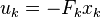
u_k = -F x_k. Op-pa. They say that for our one-dimensional example at any moment the optimal acceleration is some constant -F multiplied by the current speed? Come on, come on. But the truth is, green and red graphics are suspiciously similar to each other!

Let's try to write real equations for our 1D example.

So, we have a quality management function:



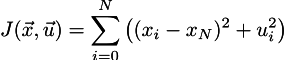
We want to minimize it, while respecting the restrictions on the connection between adjacent values ​​of the speed of our car:



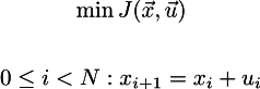
Stop-stop-stop, and what the fuck is it worth on wikipedia x_k ^ TQ x_k? After all, this is a simple x_k ^ 2 in our case, but we have (x_k-x_N) ^ 2 ?! Fir-trees, but because they assume that the final state we want to hit is the zero vector !!! WHAT IS CENSORED ABOUT THIS ON THE WHOLE WIKIPEDIA PAGE NO WORD?!

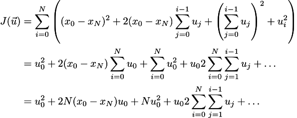
Okay, breathe deeply, calm down. Now I express all x_i in the wording of J through u_i, so as not to have restrictions. Now my variables will be only the control vector. So, we want to minimize the function J, which is written like this:



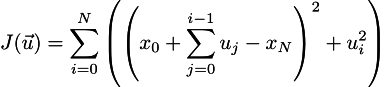
Be hurt. Now let's open the brackets (see the epigraph):



Dots here means any turbidity, which does not depend on u_0. Since we are looking for a minimum, in order to find it, we need to equate zero all partial derivatives, but first I am interested in the partial derivative with respect to u_0:



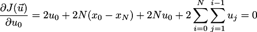
Total we get that optimal control will be optimal only when u_0 has the following expression:



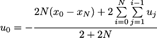
Please note that this expression includes other unknowns u_i, but there is one “but”. The joke is that I don’t want the car to accelerate to just two meters per second all the time. I gave her a minute just as obviously enough time. And I can give an hour. The term depending on u_i, if it is rough, then this is all the work on acceleration, it does not depend on N. Therefore, if N is large enough, then the optimal u_0 linearly depends only on how far x0 is from the final position!

That is, the control should look like this: we model the system, find the magic coefficient linearly connecting u_i and x_i, write it down, and then in our robot we simply make a linear proportional controller using the magic coefficient found!


To be extremely honest, I didn’t write the code, of course, until now I’ve done all of the above in mind and a little bit on paper. But this does not negate the fact that I write a lot of one-time code.

2D example

As an intuition, this is fine, but the first code I actually wrote:


Here everything is the same, only the system variables are now two: not only the speed, but also the coordinate of the machine.
So, given the initial position + initial velocity (x0, v0), I need to reach the final position (0,0), stop at the origin.
The transition from one moment to the next is carried out as x_ {k + 1} = x_k + v_k, and v_ {k + 1} = v_k + u_k.

I have commented enough on the previous code, this one should not cause difficulties. Here is the result of the work:



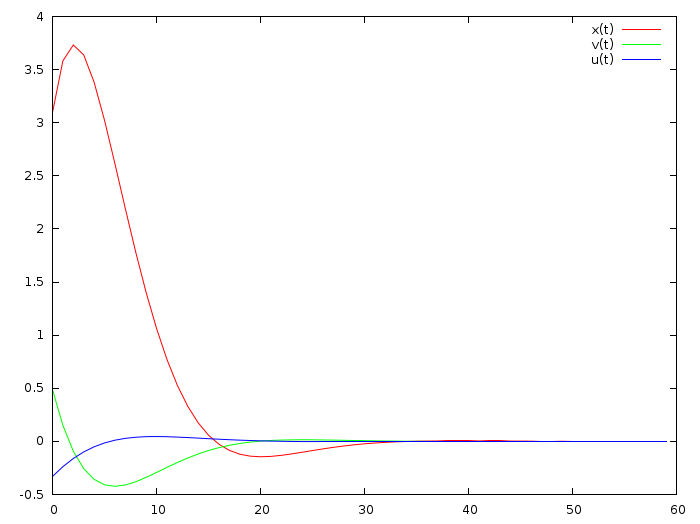
The red line is the coordinate, the green line is the speed, and the blue line is directly the position of the “gas pedal”. Based on the previous one, it is assumed that the blue curve is a weighted sum of red and green. Hmm, is this true? Let's try to count!
That is, theoretically, we need to find two numbers a and b, such that u_i = a * x_i + b * v_i. And this is nothing but a linear regression, as we did in the last article! Here is the code .

In it, I first find the curves in the picture above, and then look for such a and b, that the blue curve = a * red + b * is green.

Here is the difference between the real u_i and the ones I got by folding the green and red lines:


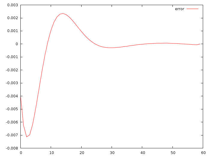
Deviation of the order of one hundredth of a meter per second per second! Cool!!! The commit I gave gives a = -0.0513868, b = -0.347324. The deviation is really small, but this is normal, I did not change the initial data.

Now let's drastically change the starting position and speed of the car, leaving the magic numbers a and b from the previous calculations.

Here is the difference between the present optimal solution and the fact that we get the most dumbest procedure, let's give it once again completely:

  double xi = x0; double vi = v0; for (int i=0; i<N; i++) { double ui = xi*a + vi*b; xi = xi + vi; vi = vi + ui; std::cout << (ui-solution[i*3+2]) << std::endl; }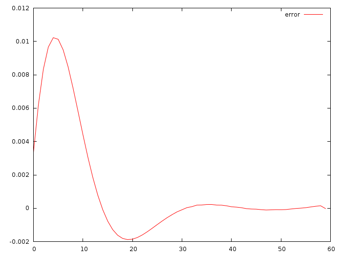 

And no differential Riccati equations that Wikipedia offered us. It is possible that I will have to read about them, but it will be later, when it burns. In the meantime, simple quadratic functions suit me more than completely.

Dry residue

Total: to use it, there will be two main difficulties:
a) find good transition matrices A and B, it will need to write kinematic equations, because, of course, everything will depend on the mass of objects and other things
b) to find good coefficients of a compromise between the goals of the fastest descent to the goal, but at the same time also without making super efforts.

If a and b do, then the method looks promising. The only thing is that it requires a complete knowledge of the state of the system, which is not always the case. For example, we don’t know the position of the segway, we can only guess about it, based on data from sensors like a gyroscope and an accelerometer. Well, that's about it, I'll tell my students next time.

So, I wanted to achieve three goals:
a) understand what lqr is
b) explain what students and you understand.
c) show you and my students that I (like most people) don’t understand shit in mathematical texts, which is sad, but not at all disastrous. We are looking for keywords to cling to, throwing out unnecessary, unnecessary methods and abstractions, and try to shove this into the framework of our current knowledge.

Hope I managed. Once again, I am not at all an expert in control theory, I have never seen her, if you have something to supplement and correct, do not hesitate.

Enjoy!