In-depth training in the garage - Two networks

This is the second article in the series about the definition of a smile on the face.

In-depth training in the garage - Data Brotherhood
In-depth training in the garage - Two networks
In-depth training in the garage - Return smiles

Calibration

So, you figured out the classifier, but you probably already noticed that the transcendental 99% somehow do not look very impressive during a combat detection test. So I noticed. Additionally, it can be seen that in the last two examples there is a very small step of the movement of windows, it will not work in life. In the present, real launch, the step is expected to look more like a picture for the first network, and there you can clearly see an unpleasant fact: no matter how well the network is looking for faces, the windows will be poorly aligned to the faces. And reducing the step is clearly not the appropriate solution to this problem for production.

Well, I thought. We found windows, but we found not exact windows, but, as it were, displaced ones. How would you move them back so that the face is in the center? Naturally, automatically. Well, since I started networking, I decided to “restore” the windows by networking too. But how?
')
The first thought came to predict three numbers by the network: by how many pixels it is necessary to shift x and y and by which constant to increase (decrease) the window. It turns out regression. But then I immediately felt that something was wrong, as many as three regressions had to be done! Yes, two of them are discrete. Moreover, they are limited by the window movement in the original image, because there is no point moving the window far away: there was another window! The last nail in the coffin of this idea turned out to be a couple of independent articles, which argued that the regression is much worse than the classification is solved by modern network methods, and that it is much less stable.

So, it was decided to reduce the regression task to the classification problem, which turned out to be more than possible, given that I need to tug the window quite a bit. For these purposes, I collected datasets, in which I took selected persons from the original dataset, shifted them to nine (including none) from different sides and increased / decreased to five different factors (including one). Total received 45 classes.

The astute reader here must be terrified: the classes turned out to be very strongly connected with each other! The result of such a classification may have little to do with reality.

To calm the inner mathematics, I gave three reasons:

1. In essence, network training is simply a search for the minimum loss function. It is not necessary to interpret it as a classification.
2. We do not classify anything, in fact, we emulate a regression! Combined with the awareness of the first point, this allows you to not focus on formal correctness.
3. That damn it works!

Since we do not classify, but emulate regression, we cannot simply take the best class and assume that it is correct. Therefore, I take the distribution of classes, which gives the network for each window, delete very unlikely (<2.2%, which is 1/45, which means that the probability is less than random), and for the remaining classes, I sum up their shifts with probabilities as coefficients and I get a regression in such a small non-basis (there would be a basis, if the classes were independent, and no basis is the same :) .
So I introduced the second calibration network into the system. She gave out a grade distribution, on the basis of which I calibrated the windows, hoping that the faces would be aligned to the center of the windows.

Let's try to train just such a network:

def build_net12_cal(input): network = lasagne.layers.InputLayer(shape=(None, 3, 12, 12), input_var=input) network = lasagne.layers.dropout(network, p=.1) network = conv(network, num_filters=16, filter_size=(3, 3), nolin=relu) network = max_pool(network) network = DenseLayer(lasagne.layers.dropout(network, p=.5), num_units=128, nolin=relu) network = DenseLayer(lasagne.layers.dropout(network, p=.5), num_units=45, nolin=linear) return network 

And here is an algorithm for calculating the offset:

 def get_calibration(): classes = np.array([(dx1, dy1, ds1), (dx2, d2, ds2), ...], dtype=theano.config.floatX) # ds --   scale min_cal_prob = 1.0 / len(classes) cals = calibration_net(*frames) > min_cal_prob #       ,     (dx, dy, ds) = (classes * cals.T).sum(axis=0) / cals.sum(axis=1) #   --   ,   --     .      ,        return dx, dy, ds 

And it works!


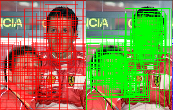
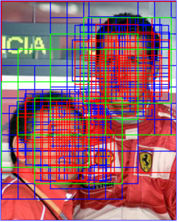
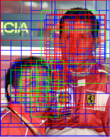
On the left, the source windows of the detection network (small), on the right, they are also calibrated. It can be seen that the windows begin to group into explicit clusters. Additionally, it helps to more effectively filter duplicates, since the windows belonging to one person intersect with a larger area and it becomes easier to understand that one of them needs to be filtered out. It also allows reducing the number of windows in production by increasing the window sliding step along the image.

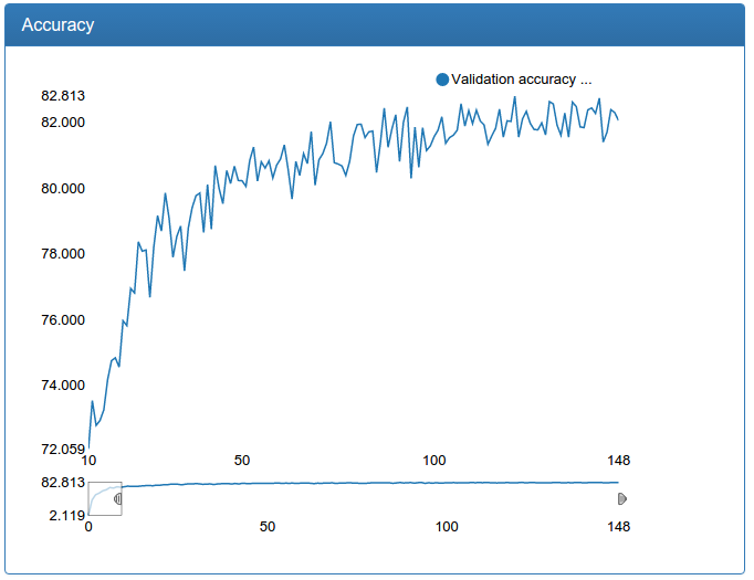
At the same time, here are the results of learning a small calibration:


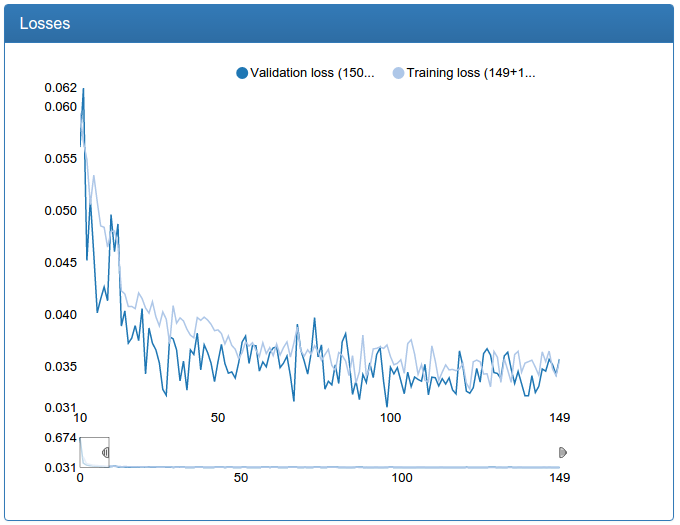
and large calibration:


and here is the largest calibration network:

 def build_net48_cal(input): network = lasagne.layers.InputLayer(shape=(None, 3, 48, 48), input_var=input) network = lasagne.layers.dropout(network, p=.1) network = conv(network, num_filters=64, filter_size=(5, 5), nolin=relu) network = max_pool(network) network = conv(network, num_filters=64, filter_size=(5, 5), nolin=relu) network = DenseLayer(lasagne.layers.dropout(network, p=.3), num_units=256, nolin=relu) network = DenseLayer(lasagne.layers.dropout(network, p=.3), num_units=45, nolin=linear) return network 

These charts should be skeptical, because we do not need a classification, but a regression. But empirical gazing shows that calibration, trained in this way, fulfills its purpose well.
I also note that for calibration, the initial data set is 45 times more than for classification (45 classes for each person), but on the other hand, it could not be completed in the manner described above simply by setting the problem. So, sausage, especially a large network, pretty.

Optimization II

Let's return to the detection. Experiments have shown that a small network does not provide the desired quality, so it is imperative to learn more. But the big problem is that even on a powerful GPU for a very long time to classify thousands of windows, which are obtained from a single photo. Such a system would simply be impossible to bring to life. In the current version there is a great potential for optimizations with cunning stunts, but I decided that they are not scalable enough and the problem should be solved qualitatively, not slyly optimizing flops. And the decision is here, before our eyes! A small network with an input of 12x12, one convolution, one pooling and classifier on top! It works very quickly, especially considering that it is possible to run the classification on the GPU in parallel for all windows - it turns out almost instantly.

Ensemble

Bind them.

So, it was decided to use not one classification and one calibration, but the whole ensemble of networks. First there will be a weak classification, then a weak calibration, then a filtering of calibrated windows, which presumably indicate one person, and then only on these remaining windows to drive a strong classification and then a strong calibration.

Later, the practice showed that it was still rather slow, so I made the ensemble as many as three levels: in the middle between the two, the "average" classification was inserted, followed by the "average" calibration and then filtering. In such a combination, the system works fast enough that there is a real opportunity to use it in production if you apply some engineering efforts and implement some tricks, just to reduce flops and increase parallelism.

Total we get the algorithm:

1. Find all the windows.
2. Check the first detection network.
3. Those that caught fire, we calibrate the first calibration network.
4. Filter overlapping windows.
5. Check the second detection network.
6. Those that caught fire, we calibrate the second calibration network.
7. Filter overlapping windows.
8. Check the third detection network.
9. Those that caught fire, we calibrate the third calibration network.
10. Filter overlapping windows.

Butchy windows

If you take steps from the second to the seventh for each window separately, it takes quite a long time: constant switching from CPU to GPU, inadequate utilization of parallelism on the video card and who knows what else. Therefore, it was decided to make pipelined logic that could work not only with separate windows, but with bats of arbitrary size. To do this, it was decided to turn each stage into a generator, and between each stage, put a code that also works as a generator, but not windows, but buoys and buffers the results of the previous stage, and accumulating a predetermined number of results (or end) gives the assembled batch further.

This system not bad (30 percent) accelerated processing during detection.

Moar data!

As I noted above in the previous article, a large detection network learns with a creak: constant sharp jumps, and even talks about it. And it's not about learning speed, as anybody who is familiar with network training thought first of all! The fact is that there is still little data. The problem is indicated - you can search for a solution! And it was immediately found: Labeled Faces in the Wild.

The combined dataset from FDDB, LFW and my personal refills has become almost three times the original. What came out of it? Less words, more pictures!

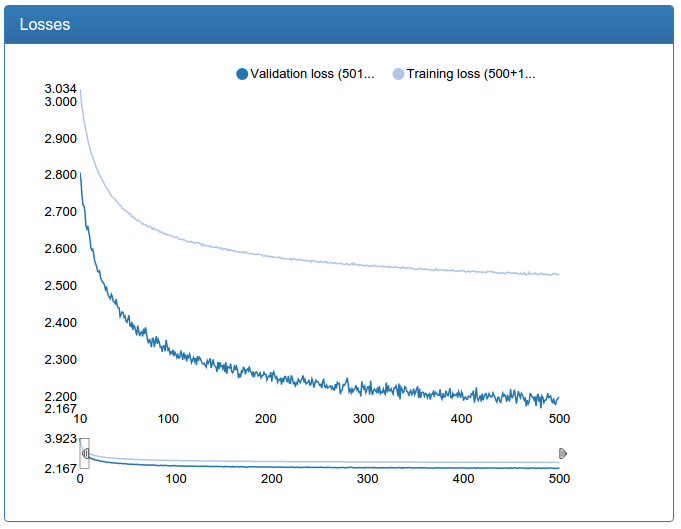
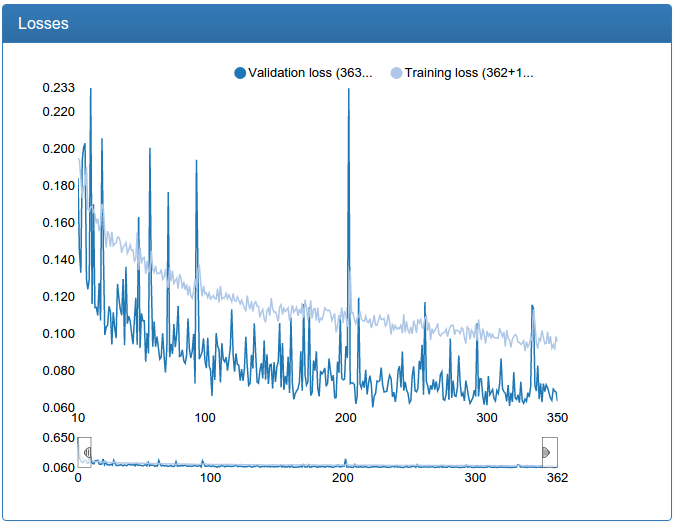
A small network is noticeably more stable, converges faster, and the result is better:


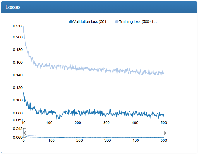
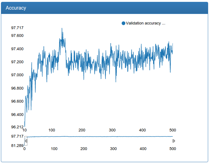
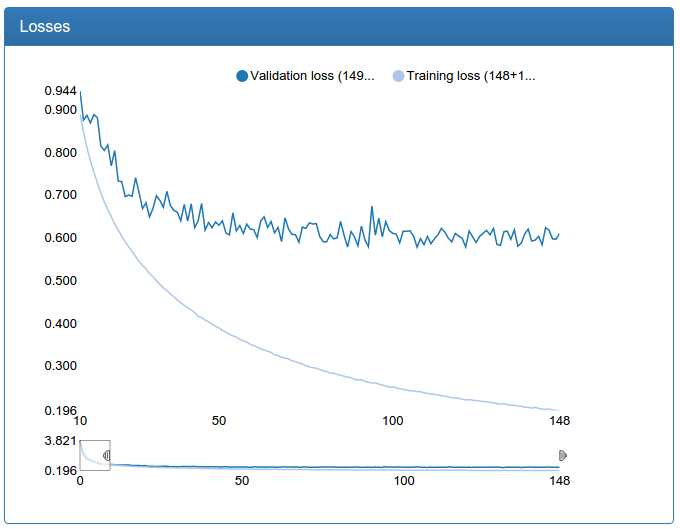
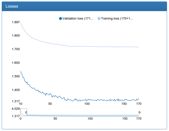
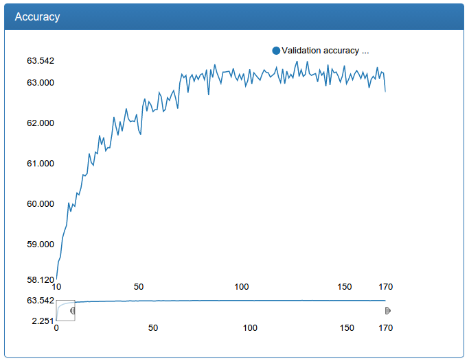
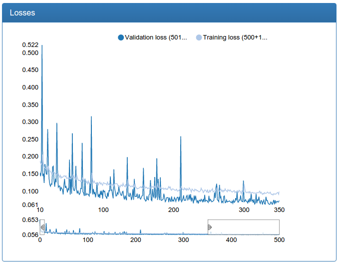
A large network is also noticeably more stable, bursts are gone, it converges faster, the result is suddenly a bit worse, but 0.17% seems to me an acceptable error:


Additionally, such an increase in the amount of data allowed us to increase the larger model for detection:


We see that the model converges even faster, to an even better result and very stable.

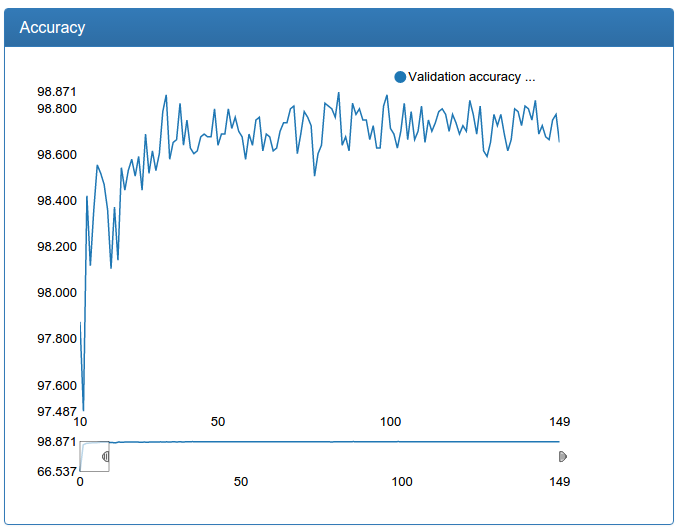
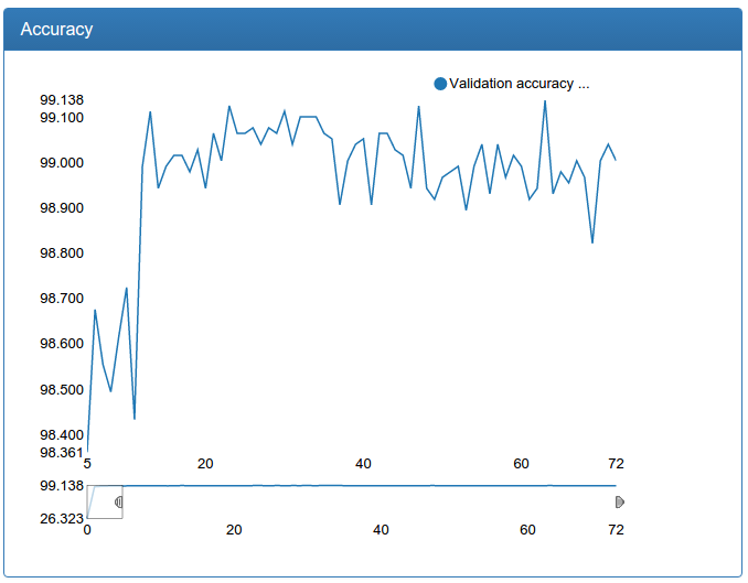
At the same time, I re-trained calibration networks on more data.

Small calibration:


and large calibration:


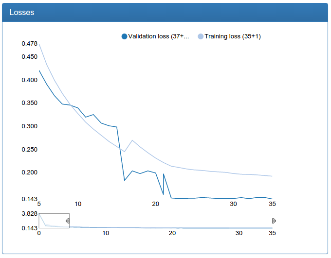
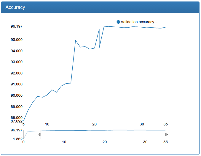
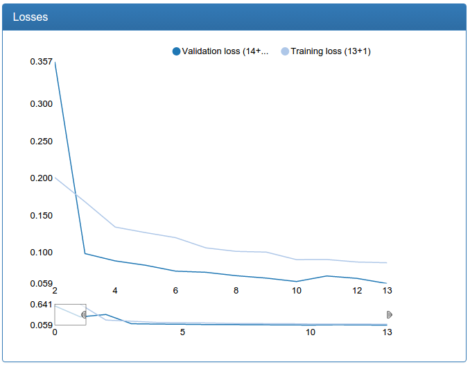
In contrast to the detection network, one can see a dramatic improvement here. This is because the original training set is not augmented and the source network suffers greatly from lack of data, as the network suffered for detection prior to augmentation.

Detection ready

A picture illustrating the entire pipeline (classification-1, calibration-1, filtering, classification-2, calibration-2, filtering, classification-3, calibration-3, filtering, global filtering, white faces from the training set):


Success!

Multi-resolution

At this point, those of you who are following the trends have probably already thought, saying that for a dinosaur, they use techniques from ancient times (4 years ago :), where are the fresh cool tricks? And here they are!

In the open spaces of arxiv.org, an interesting idea was underlined: let's consider feature maps in convolutional layers at different resolutions: it’s trite to make several inputs to the network: NxN, (N / 2) x (N / 2), (N / 4) x (N / 4) as many as you like! And serve the same square, only differently reduced.
Then, for the final classifier, all the cards are concatenated, and he seems to be able to look at different resolutions.

It was to the left, it became to the right (measured on that very average network):


It can be seen that in my case the network with several resolutions converges faster and is a little less loose. Nevertheless, I rejected the idea as not working, since the small and medium networks should not be super-accurate, and I simply increased more instead of multiresolutions with even greater success.

Batch normalization

Batch normalization is a network regularization technique. The idea is that each layer at the input accepts the result of the previous layer, in which there can be almost any tensor whose coordinates are supposedly somehow distributed. And it would be very convenient for the layer if tensors with coordinates from a fixed distribution, one for all layers, were given to the layer, then it would not need to learn the conversion invariant to the distribution parameters of the input data. Well, okay, let's insert some calculation between all the layers, which optimally normalizes the outputs of the previous layer, which reduces the pressure on the next layer and gives him the opportunity to do his job better.

This technique helped me quite well: it allowed us to reduce the probability of a dropout while maintaining the same quality of the model. Reducing the probability of a dropout in turn leads to an acceleration of the convergence of the network (and more retraining if done without normalizing the batch). Actually, literally on all the graphs you see the result: the networks quickly converge to 90% of the final quality. Before the normalization of the batches, the fall of the error was significantly more gentle (unfortunately, the results were not preserved, since there was no DeepEvent yet).

Inceptron

Of course, I could not resist digging into modern architectures and tried to train Inceptron for the classification of persons (not GoogLeNet, but a much smaller network). Unfortunately, in Theano this model cannot be correctly made: the library does not support zero-padding of arbitrary size, so I had to tear off one of the branches of the Inception module, namely the right one in this picture:


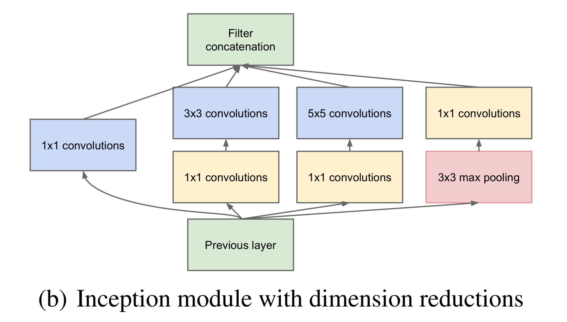
In addition, I had only three inception-modules on each other, and not seven, as in GoogLeNet, there were no preliminary exits, and there were no usual convolutionary-pooling layers at the beginning. \

 def build_net64_inceptron(input): network = lasagne.layers.InputLayer(shape=(None, 3, 64, 64), input_var=input) network = lasagne.layers.dropout(network, p=.1) b1 = conv(network, num_filters=32, filter_size=(1, 1), nolin=relu) b2 = conv(network, num_filters=48, filter_size=(1, 1), nolin=relu) b2 = conv(b2, num_filters=64, filter_size=(3, 3), nolin=relu) b3 = conv(network, num_filters=8, filter_size=(1, 1), nolin=relu) b3 = conv(b3, num_filters=16, filter_size=(5, 5), nolin=relu) network = lasagne.layers.ConcatLayer([b1, b2, b3], axis=1) network = max_pool(network, pad=(1, 1)) b1 = conv(network, num_filters=64, filter_size=(1, 1), nolin=relu) b2 = conv(network, num_filters=64, filter_size=(1, 1), nolin=relu) b2 = conv(b2, num_filters=96, filter_size=(3, 3), nolin=relu) b3 = conv(network, num_filters=16, filter_size=(1, 1), nolin=relu) b3 = conv(b3, num_filters=48, filter_size=(5, 5), nolin=relu) network = lasagne.layers.ConcatLayer([b1, b2, b3], axis=1) network = max_pool(network, pad=(1, 1)) b1 = conv(network, num_filters=96, filter_size=(1, 1), nolin=relu) b2 = conv(network, num_filters=48, filter_size=(1, 1), nolin=relu) b2 = conv(b2, num_filters=104, filter_size=(3, 3), nolin=relu) b3 = conv(network, num_filters=8, filter_size=(1, 1), nolin=relu) b3 = conv(b3, num_filters=24, filter_size=(5, 5), nolin=relu) network = lasagne.layers.ConcatLayer([b1, b2, b3], axis=1) network = max_pool(network, pad=(1, 1)) network = DenseLayer(lasagne.layers.dropout(network, p=.5), num_units=256, nolin=relu) network = DenseLayer(lasagne.layers.dropout(network, p=.5), num_units=2, nolin=linear) return network 

And I even got it!


The result is a percentage worse than the usual convolutional network, which I have previously trained, but also worthy! However, when I tried to train the same network, but out of four inception modules, it stably scattered. I still have a feeling that this architecture (at least with my modifications) is very capricious. In addition, batch normalization, for some reason, consistently turned this network into a complete raskolbas. Here I suspect a semi-handmade batch normalization implementation for Lasagne, but in general, all this made me postpone Inceptron to a bright future with Tensorflow.

By the way, Tensorflow!

Of course, I tried it too! I tried this fashionable technology on the same day, when it came out with high hopes and admiration by Google, our savior! But no, he did not justify hope. The stated automatic use of several GPUs is not in sight: on various cards, you need to place your hands on the hands; it worked only with the last kuda, which I couldn’t put on the server at that time, had a hard-coded version of libc and did not start up on another server, and it was also collected manually using a blaze, which does not work in docker containers. In short, some disappointments, although the very model of working with him is very good!

Tensorboard also turned out to be a disappointment. I don’t want to go into details, but I didn’t like everything and I started developing my monitoring called DeepEvent, screenshots from which you saw in the article.

In the next series:
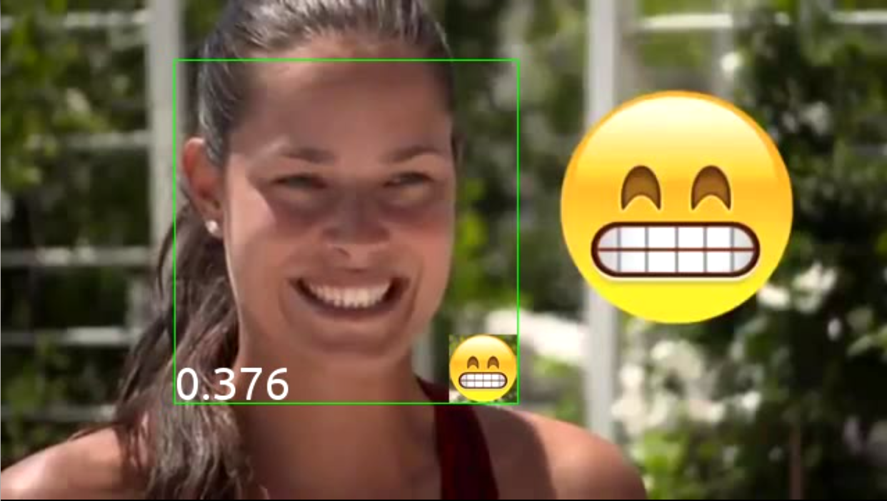
Smilies, ready system, results and, at last already, nice girls!