In the Intel Performance Primitives (IPP) library, starting from version 8.2, the transition from the internal parallelization of functions to the external one is systematically carried out. The reasons for this decision are set out in the article IPP Functions with Border Support for Image Processing in Multiple Streams .

In this post, we will consider the functions that implement the filter with the final response - FIR filter (Finite Impulse Response).

FIR filter

Filters are one of the most important areas in digital signal processing. And, of course, the IPP library has an implementation of most of the classes of these filters, including the FIR (finite impulse response) filter. A detailed description of the FIR filters can be found in numerous literature or in Wikipedia, but if briefly, in a few words, the FIR filter simply multiplies several previous samples and the current sample of the input discrete signal by their corresponding coefficients, adds these products and obtains the current output sample. Or a little more formally: the FIR filter transforms the input vector X with a length of N samples into the output vector Y with a length of N samples too by multiplying K samples of the input vector with the corresponding K coefficients H and subsequent summation. The number of coefficients K is called the order of the filter.


Fig. 1. FIR filter
')
Here:
tapsLen is the filter order,
numIters is the length of the vector.
The figure is taken from the documentation for the IPP library, so the terminology used in IPP is used.
Visually, you can imagine the FIR filter as follows.


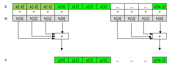
Fig. 2. FIR filter schematically

As we see, here the order of the filter K is 4 and we simply multiply the 4 coefficients h of the filter by 4 samples of the vector x, add and write the sum into one sample of the output vector y. Note that the filter coefficients h [3], h [2], h [1], h [0] are stored in the memory in the reverse order with respect to x and y, in accordance with the generally accepted formula in Fig. one

Delay line

Since the FIR filter is an ordinary convolution, to obtain an output vector with a length of N samples, you need N + K-1 input samples, where K is the kernel length. The first K-1 samples will be referred to as the “delay line”. In fig. 2 they are numbered x [-3], x [-2], x [-1]. The data supplied to the function can be quite large, as a result of which it can be broken up into separate sequentially processed blocks. For example, if it is an audio signal, then it can be buffered by the operating system, if it is data from an external device, then it can come in portions of the communication line. Also, data can be processed through the buffer and in the application itself, since the amount of possible data is not known in advance. In this case, the working buffer is allocated some fixed length, for example, so that they fit into the cache of a certain level and then all data passes through this buffer in chunks. In all such cases, the delay line is very useful. It helps to very simply “glue” the data into one continuous stream in such a way that there is no edge effect of breaking the data into blocks.

IPP API

Years of experience in using the IPP library have revealed that it is necessary to modify the API FIR filters to meet the following requirements:

• it would be possible to process the vector in successive blocks;
• there would be no hidden memory allocation;
• vector processing in different streams would be supported;
• It was allowed in-place mode, ie the input vector is also an output.

In order to fulfill all these requirements at the same time, the concepts of “input” and “output” delay lines were introduced, after which the API began to look like this.

This API follows the standard scheme used in IPP. First, with the help of the ippsFIRSRGetSize function , the size of the memory for the function context and the work buffer are requested. Next, the function ippsFIRSRInit is called , to which the filter coefficients are fed. This function initializes the internal data tables in the pSpec structure, speeding up the processing of the ippsFIRSR processing function. The content of this structure does not change during the operation of the function, which is reflected in its name Spec, therefore it can be used simultaneously by several threads for more efficient use of memory. The pBuf parameter is a working and modifiable function buffer, so each thread must have its own working buffer.

The suffix SR stands for single rate, and is used for uniformity with MR (multi rate) filters, the description of which can be a whole separate article. The numIters parameter is also borrowed from the MR filters and in our case simply means the length of the vector.
The beginning of the block x [0] being processed is indicated by the pSrc parameter.
Now consider what meaning is embedded in the parameters pDlySrc and pDlyDst.


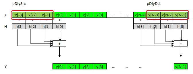
Fig. 3. "Input" and "Output" delay lines

As mentioned earlier, the need for x [-3], x [-2], x [-1] comes from the convolution formula. These elements are called the “input delay line” pDlySrc. And the samples x [N-3], x [N-2], x [N-1] are the “tail” of the processed vector, i.e. last k-1 items. They are called the “output delay line” pDlyDst. For the next block, they will respectively be the input line, and so on.
The input delay line pDlySrc can point to k-1 samples to the left of x [0], to some other buffer or equal to NULL. In the case of NULL, it is assumed that all elements of the input delay line are equal to 0. This is convenient for the initial block when there is no incoming data yet.
At the address pDlyDst, the block “tail” is recorded, i.e. k-1 last counts. If the value is NULL, then nothing is written.

Such a mechanism of two delay lines allows parallelizing the processing of a vector, even in the case of in-place mode, i.e. when the vector is overwritten. To do this, simply copy the “tails” of the blocks into separate buffers and submit them as an input line to each stream. An example of the code used in the article is given at the end of a single listing.

An example of using the Lowpass IPP FIR filter.

Consider, for example, how to use the IPP FIR filter in order to leave only the low-frequency component of the signal.
To generate the original unfiltered signal, we will use the special IPP function Jaehne, which implements the formula
pDst [n] = magn * sin ((0.5πn2) / len), 0 ≤ n <len
This feature is the workhorse on which many IPP functions are tested. The generated signal will be recorded in the simplest .csv file and draw pictures in Excel. The original signal looks like this.


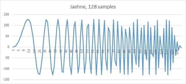
Fig. 4. 128 Jaehne Signal Counts

Consider, for example, a filter of order 31. To generate coefficients, use the IPP function ippsFIRGenLowpass_64f . The function calculates the coefficients only in double, so they are converted to float. See the function code firgenlowpass () in the appendix. After calling this function, the buffer size, initialization and call of the main function ippsFIRSR are calculated, and its performance is also measured.
After applying the lowpass filter, the low-frequency component remained in the signal. Note that the phase is shifted, but this already follows from the property of the FIR filters themselves and does not apply to the IPP library.


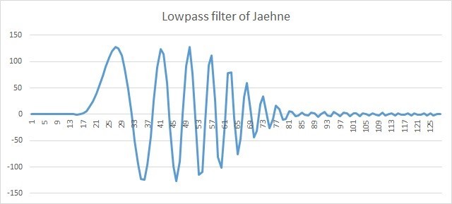
Fig. 5. 128 Jaehne signal samples after lowpass filter

In these figures, the FIR filter processes 128 samples, while 30 samples of the input delay line are set to 0, indicating pDlySrc = NULL. The output line we also do not need pDlyDst = NULL.

Multi-threaded version performance

The IPP library has in its title the word performance (performance), which is put at the forefront. Therefore, we measure the performance of the ippFIRSR function on the processor with support for AVX2. After that, we implement the following multi-threaded code using OpenMP, measure it and then reduce the measurement results into one graph.
The FIR Filter API was designed in such a way that splitting a vector into several streams was simple and logical, as shown in the figure:


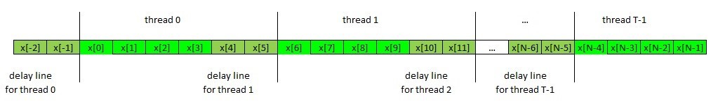
Fig. 6. Splitting the source vector between threads

The following way of splitting a vector between threads is implied, see the fir_omp function.


Consider what this code does. So, we received the next portion of the signal x [0], ..., x [N-1], which needs to be processed by the filter, and with it a pointer to the input and output delay lines or in other words the “tail” of the previous portion and the buffer, where should be placed “tail” of the current portion. We want to speed up the filtering process and break the processing of this portion into T = NTHREADS blocks corresponding to the number of threads. To do this, we just need to correctly specify the input and output lines, and also allocate our own working buffer for each stream.

For the 0th stream, the input delay line when calling ippsFIRSR is the very “tail” of the previous batch, and for all others, the pointer to the block shifted by order-1 elements is given as the input line. And only the last stream records the “tail” of the portion.

The above approach implies that the resulting vector is written to a different address than the original vector, if the data is overwritten, then the delay lines should be copied to separate buffers.

The graph shows the performance of single-threaded and multi-threaded versions for 4 31-order filter threads on an AVX2 processor supporting Intel® Core (TM) i7-4770K 3.50Ghz. For FIR filters, the unit of measure is cpMAC, i.e. the number of ticks for the operation Multiply + Add
cpMAC = (function execution time) / (vector length * filter order)


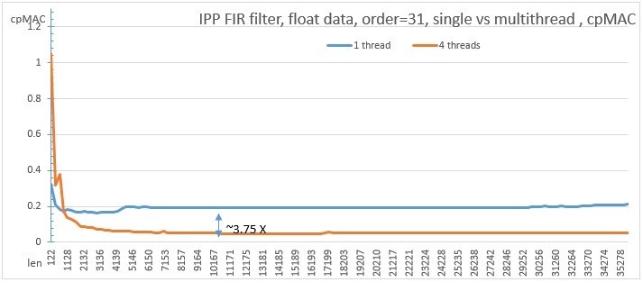
Fig. 7. Comparison of performance of single-threaded and multi-threaded versions of FIR filter

It can be seen that the function is very well scaled, and the multi-threaded version works approximately 3.7 times faster on fairly long vectors than single-threaded, which corresponds very well to 4 threads. The criterion for switching between single- and multi-threaded versions now, with the new API, can be chosen experimentally for a specific machine, unlike the previous one, where the criterion was rigidly sewn into the code and the function was parallel from the inside.

Comparison of direct and FFT implementations

In digital signal processing, the mutual correspondence between convolution and Fourier transform is widely used.
In addition to direct implementations, IPP FIR filters also have an implementation via FFT, and the cpMACs obtained in this case sometimes exceed the theoretically possible for a given cpu and direct algorithm, which users sometimes write about in forums, believing that calculations go through FFT.

Now, in order to specify what type of algorithm to use, you should use one of the values ​​of the algType parameter - ippAlgDirect ippAlgFFT, ippAlgAuto. The last parameter means that the function selects an algorithm according to a fixed criterion for the cpu used, and it may not always be optimal.

Consider the performance on the same CPU filter of different orders for a vector length of 1024 and 128 samples using a direct algorithm and FFT implementation.


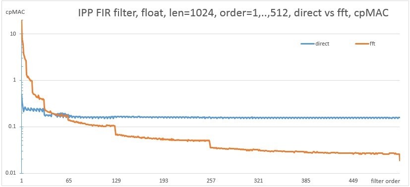
Fig. 8. Comparison of performance of direct and fft implementations for a length of 1024 samples


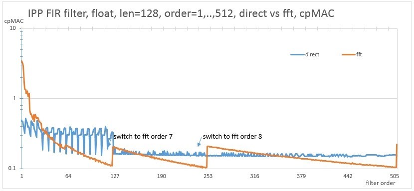
Fig. 9. Comparison of the performance of direct and fft implementations for a length of 128 samples

Steps are characteristic for FFT implementation. This is explained by the fact that for filters of several close orders the FFT of the same order is used, and when the transition goes to the next FFT order, the performance changes. For maximum performance, you should use the algorithm that lies on the graph below. The proposed API allows you to implement an example that will run both versions of the algorithm for measurement on a specific machine, and select the best of them. The picture will look something like this. This picture shows a two-dimensional space with a size of 1024x1024, where along the X axis the order of the filter and along the Y axis the length of the vector. Green color means that the fft algorithm is faster than the direct version. The characteristic straight lines at the bottom of the figure correspond to fig. 9, where the fft option works for some time more slowly, after the transition to the next order.


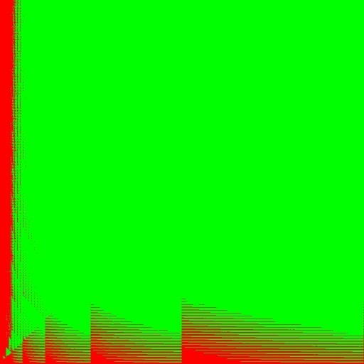
Fig. 10. Comparison of direct and fft performance of an IPP FIR implementation of a filter float in filter order space X vector length of 1024 x 1024

It can be seen that the drawing is quite complicated and it is not so easy to interpolate inside the IPP under an arbitrary platform. In addition, this pattern may vary on a specific machine. In addition to the choice between direct and fft code, you can add another dimension in the form of the number of threads and in this way you will get a multi-layered image. The proposed API again allows you to choose the best option for this platform in this case.

Conclusion

Introduced in IPP 9.0 API, FIR filters allow using them in applications even more efficiently, choosing the best option between direct and fft algorithms, as well as parallelizing each of the selected options. In addition, the IPP library is completely free and available for download at this link Intel Performance Primitives (IPP).

Application. Sample code measuring IPP FIR filter performance