Connectivity components in a dynamic graph in one pass

People meet, people quarrel, add and remove friends in social networks. This post is about mathematics and algorithms, beautiful theory, love and hate in this unstable world. This post is about searching for connected components in dynamic graphs.

The big world generates big data. So a big graph fell on our head. So big that we can keep in memory its vertices, but not edges. In addition, there are updates regarding the graph - which edge to add, which one to delete. We can say that every such update we see for the first and last time. In such conditions it is necessary to find the components of the connectivity

Search in depth / width here will not pass simply because the entire graph in the memory does not hold. A system of disjoint sets could greatly help if the edges in the graph were added. What to do in the general case?
')

Task . Dan undirected graph $G$ on $n$ tops. Initially, the graph is empty. The algorithm comes a sequence of updates. $p_1, p_2, \ dots, p_m$ , which can be read in a given order exactly once. Each update is a command to remove or add an edge between a pair of vertices. $u_i$ and $v_i$ . It is guaranteed that at any point in time between a pair of vertices more edges than they are will not be deleted. After reading the sequence, the algorithm should output all connected components with a probability of success. $0.99$ . Permitted to use $O (n \ log ^ c n)$ memory where $c$ - some constant.

The solution of the problem consists of three ingredients.

Incidence matrix as a representation.
The method as an algorithm.
$L_0$ Sampling as optimization.

You can see the implementation on the githaba: link .

Incidence Matrix as Representation

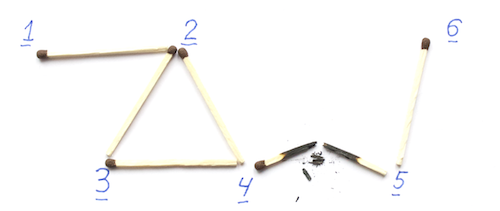
The first data structure for the storage of the graph will be extremely non-optimal. We will take the incidence matrix $A$ size $n \ times \ binom {n} {2}$ , which will mostly be zeros. Each row in the matrix corresponds to a vertex, and a column corresponds to a possible edge. Let be $u & lt; v$ . For a pair of vertices $u, v$ connected by an edge, we define
$A_ {u, (u, v)} = 1$ and $A_ {v, (u, v)} = -1$ , otherwise the values are zero.

As an example, look at the graph in the picture below.

For him, the incidence matrix will look like this.

$\ begin {array} {r | ccccccccccccccc} A & amp; (1, 2) & amp; (1, 3) & amp; (1, 4) & amp; (1, 5) & amp; (1, 6) & amp; (2, 3) & amp; (2, 4) & amp; (2, 5) & amp; (2, 6) & amp; (3, 4) & amp; (3, 5) & amp; (3, 6) & amp; (4, 5) & amp; (4, 6) & amp; (5, 6) \\ hline 1 & amp; +1 & amp; 0 & amp; 0 & amp; 0 & amp; 0 & amp; 0 & amp; 0 & amp; 0 & amp; 0 & amp; 0 & amp; 0 & amp; 0 & amp; 0 & amp; 0 & amp; 0 \\ 2 & amp; -1 & amp; 0 & amp; 0 & amp; 0 & amp; 0 & amp; +1 & amp; +1 & amp; 0 & amp; 0 & amp; 0 & amp; 0 & amp; 0 & amp; 0 & amp; 0 & amp; 0 \\ 3 & amp; 0 & amp; 0 & amp; 0 & amp; 0 & amp; 0 & amp; -1 & amp; 0 & amp; 0 & amp; 0 & amp; +1 & amp; 0 & amp; 0 & amp; 0 & amp; 0 & amp; 0 \\ 4 & amp; 0 & amp; 0 & amp; 0 & amp; 0 & amp; 0 & amp; 0 & amp; -1 & amp; 0 & amp; 0 & amp; -1 & amp; 0 & amp; 0 & amp; 0 & amp; 0 & amp; 0 \\ 5 & amp; 0 & amp; 0 & amp; 0 & amp; 0 & amp; 0 & amp; 0 & amp; 0 & amp; 0 & amp; 0 & amp; 0 & amp; 0 & amp; 0 & amp; 0 & amp; 0 & amp; +1 \\ 6 & amp; 0 & amp; 0 & amp; 0 & amp; 0 & amp; 0 & amp; 0 & amp; 0 & amp; 0 & amp; 0 & amp; 0 & amp; 0 & amp; 0 & amp; 0 & amp; 0 & amp; -1 \\ \ end {array}$

The naked eye can see that this view has a serious drawback - the size $O (n ^ 3)$ . We optimize it, but later.

There is also an implicit advantage. If you take a lot of vertices $S$ and add all matrix row vectors $A$ that match $S$ , then the edges between the vertices $S$ only those connecting will be reduced $S$ and $V \ backslash s$ .

For example, if you take a lot $S = \ {3, 4, 5 \}$ and put the corresponding vectors, we get

Non-zero values are at the edges $(2, 3)$ , $(2, 4)$ and $(5, 6)$ .

Shrinking the graph as an algorithm

Understand what a rib is. Here we have two peaks $u$ and $v$ there is a rib between them. Of $u$ and $v$ there may be other edges. Stiffen rib $(u, v)$ this is the procedure when we merge the vertices $u$ and $v$ in one let's say $w$ , rib $(u, v)$ we delete, and all remaining edges, incident $u$ and $v$ , we lead to the new peak $w$ .

An interesting feature: in terms of the matrix of incidence, to tighten the edge $(u, v)$ it is enough to add the corresponding row vectors. Edge itself $(u, v)$ shrink, only those that go outside will remain.

Now the algorithm. Take a graph and for each non-isolated vertex we choose a neighbor.

We pull the corresponding edges.

Repeat iteration $\ log n$ time.

Note that after each iteration of the connection of the connected components of the new graph are one-to-one mapped to the components of the old. We can even mark which vertices have been merged into the resulting vertices, in order to restore the answer later.

Note also that after each iteration, any connected component of at least two vertices is reduced at least two times. This is natural, since at least two vertices of the old one were merged into each vertex of the new component. So after $\ log n$ iterations in the graph will remain only isolated vertices.

We search through all isolated vertices and restore the answer in the history of mergers.

$L_0$ -sampling as optimization

Everything would be great, but the above algorithm works in terms of time and memory. $O (n ^ 3)$ . To optimize it, we will construct a sketch - a special data structure for a compact representation of row vectors.

From the sketch you need three properties.

First, compactness. If we build a sketch for a vector $a$ size $O (n)$ then the sketch itself $\ sigma (a)$ must be sized $O (\ log ^ c n)$ .

Secondly, sampling. At each iteration of the algorithm, we need to choose a neighbor. We want a way to get the index of at least one non-zero element, if there is one.

Third, linearity. If we built for two vectors $a$ and $b$ sketches $\ sigma (a)$ and $\ sigma (b)$ . Must be an effective method, get a sketch $\ sigma (a + b) = f (\ sigma (a), \ sigma (b))$ . This will help tighten the ribs.

We will use the solution of the problem. $L_0$ -sampling.

Task. Dan vector zero vector $a = \ langle a_1, a_2, \ dots, a_n \ rangle$ dimensions $n$ . Algorithm sequence comes from $m$ view updates $(i, \ Delta)$ : add $\ Delta$ to value $a_i$ . $\ Delta$ can be either positive or negative integer. The resulting vector at some positions may have non-zero values. These positions are denoted by $I$ . It is required to issue any position from $I$ equally likely. All updates need to be processed in one pass, you can use $O (\ log ^ c n)$ of memory. It is guaranteed that the maximum value in $a_i$ fit in $O (\ log n)$ bit.

1-sparse vector

To begin, we will solve a simpler problem. Suppose we have a guarantee that the final vector contains exactly one nonzero position. We say that such a vector is 1-sparse. We will support two variables $S_0 = \ sum_i a_i$ and $S_1 = \ sum_i i \ cdot a_i$ . Maintaining them is simple: on each update we add to the first $\ Delta$ to second $i \ cdot \ Delta$ .

Denote the desired position by $i '$ . If it is only one, then $S_0 = a_ {i '}$ and $S_1 = i '\ cdot a_ {i'}$ . To find a position, we consider $i '= S_1 / S_0$ .

You can probabilistically check whether the vector is 1-sparse. For this we take a prime number $p & gt; 4 \ cdot n$ random integer $z \ in [0, p)$ and calculate the variable $T = \ sum_i a_i \ cdot z ^ i% p$ . The vector passes the 1-sparsity test if $S_0 \ neq 0$ and $T = S_0 \ cdot z ^ {S_1 / S_0}$ .

Obviously, if the vector is really 1-sparse, then

$T = \ sum_i a_i \ cdot z ^ i = a_ {i '} \ cdot z ^ {i'} = S_0 \ cdot z ^ {S_1 / S_0}$

and he will pass the test. Otherwise, the probability of passing the test is not more than $0.25$ (actually, maximum $n / p$ ).

Why?

In terms of a polynomial, a vector passes the test if the values of a polynomial

$p (z) = \ sum_i a_i \ cdot z ^ i - S_0 \ cdot z ^ {S_1 / S_0}$

randomly selected point $z$ equals zero. If the vector is not 1-sparse, then $p (z)$ is not identically zero. If we passed the test, we guessed the root. The maximum degree of a polynomial is $n$ means no more roots $n$ so the probability of guessing them is no more $n / p$ .

If we want to increase the accuracy of verification to an arbitrary probability $1 - \ delta$ , then you need to calculate the value $T$ on $O (\ log \ delta ^ {- 1})$ random $z$ .

$s$ -frame vector

Now we will try to solve the problem for $s$ - sparse vector, i.e. containing no more $s$ nonzero positions. We will need hashing and the previous method. The general idea is to restore the entire vector, and then select some element randomly.

Take a random 2-independent hash function $h: [n] \ rightarrow [2s]$ . This is such a function, which distributes two arbitrary different keys equally independently.

More about hash functions

The algorithms have two fundamentally different approaches to hash functions. The first is based on the fact that the data is less random, and our favorite hash function will mix them correctly. The second is that an evil adversary can pick up data, and the only chance to save the algorithm from unnecessary computation and other problems is to choose a hash function randomly. Yes, sometimes it can work poorly, but we can measure how bad it is. Here we are talking about the second approach.

The hash function is selected from the family of functions. For example, if we want to stir all the numbers from

before $p - 1$ you can take random $a$ and $b$ and determine the hash function

$h_ {a, b} (x) = a \ cdot x + b \ text {mod} p.$

Functions for all possible $a, b \ in [p]$ set the family of hash functions. Randomly select the hash function - it is essentially random to select those $a$ and $b$ . They are usually chosen equiprobably from the set $[p]$ .

The remarkable property of the example above is that any two different keys are randomly distributed independently. Formally, for any different $x_1, x_2 \ in [p]$ and any, possibly the same, $y_1, y_2 \ in [p]$ probability

$\ textbf {Pr} \ left [h (x_1) = y_1 \ text {and} h (x_2) = y_2 \ right] = p ^ {- 2}.$

This property is called 2-independence. Sometimes, the probability may not be $p ^ {- 2}$ , but $p ^ {- 2} \ pm \ varepsilon$ where $varepsilon$ some kind of reasonably small value.

There is a 2-independence generalization - $k$ -independence. This is when the function distributes not 2, $k$ arbitrary keys regardless. Polynomial hash functions with $k$ random coefficients have this property.

$p (x) = \ sum_ {i = 0} ^ {k - 1} a_i \ cdot x ^ i \ text {mod} p$

Have $k$ Independence is one unpleasant property. With growth $k$ function takes up more memory. This property does not depend on any particular implementation, but simply a general information property. Therefore, the less independence we can do, the easier it is to live.

Take a hash table size $2s$ . In each cell of the table, there will be an algorithm for a 1-sparse vector. When we receive an update $(i, \ Delta)$ , we send this update to the algorithm in the cell $h (i)$ .
It can be calculated that for a single cell, the probability that there will be a collision at least along two non-zero coordinates will be no more than $0.4$ .

Why?

The probability that another element does not fall into the cell to us $(1 - 1 / 2s)$ . The probability that everyone will not get to us: $(1 - 1 / 2s) ^ {s- 1}$ . The probability that at least someone will fall $1 - (1 - 1 / 2s) ^ {s - 1}$ . You may notice that this function is monotonically increasing. I'll just bring a picture here:

In the limit, the function gives the value $1 - e ^ {- 0.5} \ leq 0.4$ .

Suppose we want to restore all coordinates with probability of success. $1 - \ delta$ or with probability of failure $\ delta$ . Take not one hash table, but immediately $k = O (\ log (s \ cdot (\ delta / 2) ^ {- 1}))$ . It is easy to understand that the probability of failure in decoding a particular coordinate will be $(\ delta / 2) / s$ . The probability of failure in decoding at least one of $s$ coordinates $\ delta / 2$ . If the total decoding for 1-sparse vectors works with the probability of failure $\ delta / 2$ then we won.

The final algorithm is as follows. Take $O (\ log (s \ cdot \ delta ^ {- 1}))$ hash table size $2s$ . Each cell of the algorithm will have its own decoder for a 1-sparse vector with the probability of failure $\ delta / 2 k s$ .

Every update $(i, \ Delta)$ processed in each hash table separately by the algorithm in the cell $h_j (i)$ .

Upon completion, we extract from all successfully completed 1-decoders by coordinate and merge them into one list.

The maximum in the general table will be $k \ cdot s$ affected 1-decoders. Therefore, the total probability that one of the 1-decoders will not work correctly will not exceed $k s \ cdot \ delta / 2 ks = \ delta / 2$ . Also, the probability that at least one coordinate will not be restored does not exceed $\ delta / 2$ . Overall, the probability of failure of the algorithm $\ delta$ .

Another hash for general case

Last step in $L_0$ -sampling, is to understand what to do with the general case. We will use hashing again. Take $O (s)$ -independent hash function $h: [n] \ rightarrow [2 ^ k]$ for some $2 ^ k \ geq n ^ 3$ .

Let's say that the update $(i, \ Delta)$ is an $j$ interesting if $h (i) \ text {mod} 2 ^ j = 0$ . In other words, in binary record $h (i)$ contains $j$ zeros at the end.

Run the algorithm for $s$ -frame vector in parallel by $\ log n$ levels. At the level $j$ we will take into account only $j$ - interesting updates. It is easy to understand that the more $j$ the less chance (and chances $2 ^ {- j}$ ) have the update be taken into account.

Find the first level with the highest $j$ where there came at least some updates, and try to restore it. If the recovery is successful, we will return the randomly selected item.

There are several points that I want to briefly pay attention to.

First, how to choose $s$ . In general, a vector may have more than $s$ non-zero positions, but with every increase $j$ per unit, mat. the expectation of non-zero positions drops exactly 2 times. You can choose a level at which the expectation will be between $s / 4$ and $s / 2$ . Then from Chernov and $O (s)$ independence of the hash function, the probability that the vector will be zero or have more than $s$ nonzero positions will turn out to be exponentially small.

This determines the choice $s = O (\ log \ delta ^ {- 1})$ where $\ delta$ - the permissible probability of failure.

Secondly, from $O (s)$ -independence of the hash function implies that for any position the probability to pass the filter will be equal. Insofar as $s$ - sparse vectors, we can already recover, then getting a uniform distribution is already trivial.

So we learned how to choose a random non-zero position according to a uniform distribution.

Mix, but do not shake

It remains to understand how to combine everything. We know that in the graph $n$ vertices. For each vertex, or rather, each row vector in the incidence matrix, we will $\ log n$ sketches $\ sigma_1 (A_v), \ sigma_2 (A_v), \ dots, \ sigma _ {\ log n} (A_v)$ for $L_0$ -sampling. On $i$ th iteration algorithm we will use for sampling $i$ sketches

When adding an edge $(u, v)$ add vertices to all sketches $u$ and $v$ corresponding +1 and -1 respectively.

When the ribs are over and we are asked about the components, we will run the tightening algorithm. On $i$ iteration through $L_0$ -sampling from the sketch $\ sigma_i (v)$ find a neighbor to each vertex. To pull the edge $(u, v)$ , we add all the sketches corresponding $u$ and $v$ . At each new vertex we will save the list of vertices that were merged into it.

Everything. In the end, just go through the isolated peaks, the history of mergers restore the answer.

Who is to blame and what to do again

In fact, the topic of this post has arisen for a reason. In January, Ilya Razenshtein (@ilyaraz), a graduate student at MIT, came to us at Peter's CS Club and talked about algorithms for big data. There was a lot of interesting (see course description ). In particular, Ilya managed to tell the first half of this algorithm. I decided to finish the job and tell the whole result on Habré.

In general, if you are interested in mathematics related to computational processes aka Theoretical Computer Science, come to our Academic University in the direction of Computer Science . Inside they will teach complexity, algorithms and discrete mathematics. The real science will start from the first semester. You can get out and listen to courses in the CS Club and CS Center . If you are not from St. Petersburg, there is a hostel. A great chance to move to the Northern Capital.

Apply , get ready and come to us.

Sources

Source: https://habr.com/ru/post/276563/

All Articles