How are the packages for checking the quality of random sequences?
The question of obtaining random and pseudo-random sequences is always of great interest [ 1 ] [ 2 ] [ 3 ] [etc.]. Frequently [ 1 ], [ 2 ] [, etc.] are also referred to as statistical test packages, such as NIST, DieHard, TestU01.
In the comments to the articles on Habrahabr there are questions about how these packages receive the final figures. In general, there is nothing difficult - it's just statistics. If the reader is interested in the magic of obtaining these figures, then I ask for a cat, there are a lot of beeches and formulas.
If possible, I want to make the presentation as clear as possible for an unprepared user, so please forgive for some inaccuracies and omitted definitions.
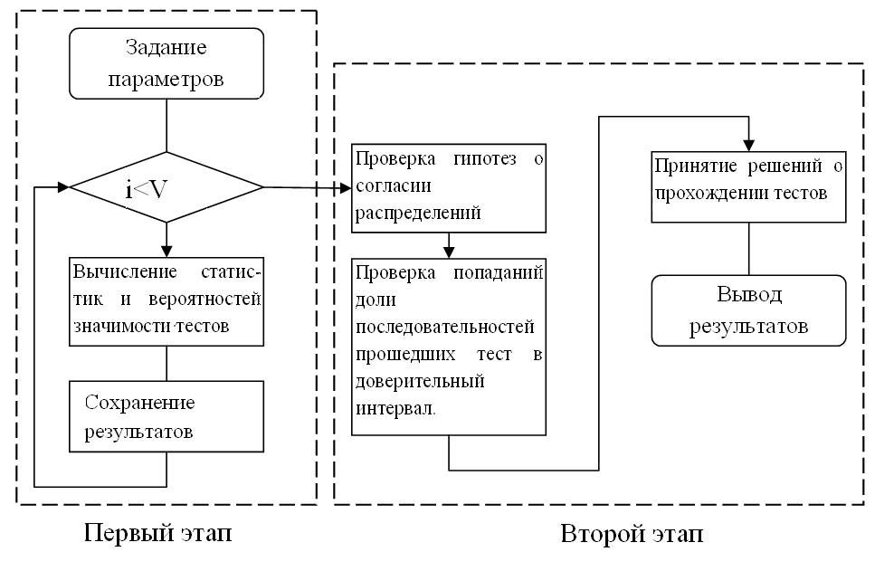
Statistical sequence analysis, as a rule, takes place in two stages.
Schematically, this process can be represented like this:
')
The goal of each test is to test the hypothesis that the sequence under investigation has a uniform distribution. Speaking more strictly, each sign random sequence
  should have a uniform probability distribution:
 %20%3D%201%2F2%2C%20x%5Cin%5C%7B0%2C1%5C%7D) . This hypothesis is denoted by
. This hypothesis is denoted by  (they say the null hypothesis).
And from where do the formulas for test statistics appear? Let's take a look at the example of a frequency test from the NIST package.
Each statistical test tests some assumption about a particular property that a random sequence must have that satisfies the hypothesis. .
For the frequency test from the NIST test suite, this assumption is the statement: “If the sequence satisfies the hypothesis then the number of zeros and ones in this sequence should be about the same. "
If we find the sum of characters of the sequence under study, then the final result will be a random variable, let's call it :
:  . According to the central limit theorem, the random variable in our assumptions should have a distribution close to the normal distribution with the expectation
  and standard deviation
  .
.
Since we are interested in the deviation of the number of units (zeros) from the expectation, we will consider a random variable . Divide it into so that the variance of the obtained value equals 1. And we take all this in absolute value, since we are not interested in the sign of the deviation. What happened?
 .
.
The result was a random variable depending on the sequence under study. The distribution function of this random variable under the hypothesis assumption equals:
%3DP(S%5Cle%20x)%3D2%5CPhi%20(x)-1%2Cx%3E0) (zero for all x),
(zero for all x),
Where) - function of standard normal distribution.
- function of standard normal distribution.
The value of S calculated for a particular sequence X is called "statistics". If you look at the NIST test descriptions, you can find this particular formula for calculating test statistics.
Using the same reasoning, formulas for other tests appear.
It is necessary to determine whether the statistics S deviates significantly from zero or not.
Deviation should not be "too" big. The word "too" does not give specific instructions for action. Therefore, we choose some critical level - probability of mistakenly rejecting the hypothesis . To this matches critical value
  which defines a critical area. We demonstrate this in the pictures:
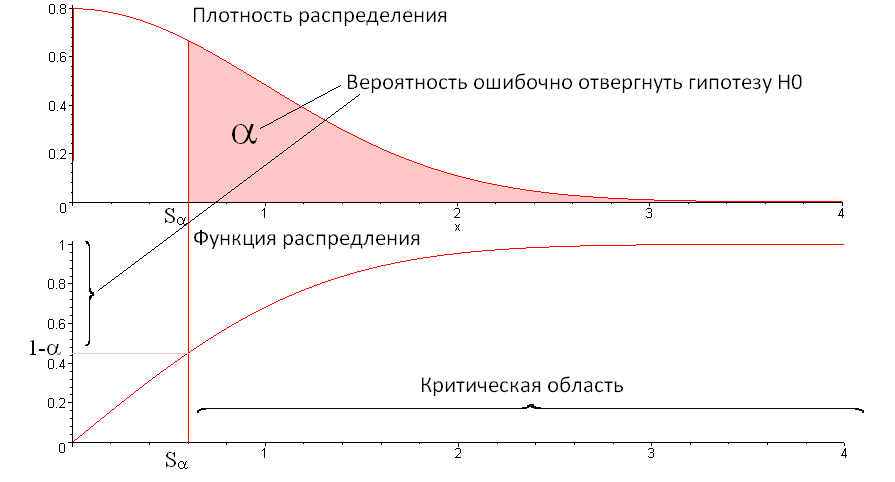
In other words represents the boundary for deciding whether a sequence passed the test or not. If value  , then we believe that the sequence is “good” - passed the test. If S is in the critical area
  , then we consider the sequence is bad - did not pass the test.
In packages of statistical studies, another equivalent decision-making method is often used. According to statistics, S calculates the probability of significance p, which is equal to:) . This value will be less than or equal to
. This value will be less than or equal to  , only in case of hit of S in critical area.
Usually choose in the range from 0.01 to 0.001. The more the more sequences will be rejected.
Immediately the question arises: "How to reject a generator of (pseudo) random numbers, if part of the sequences is bad, and part is good?"
In fact, any random sequence generator will always generate part of the sequences that fail the test. I would even say that if all the sequences pass the test, it is very suspicious.
At the first stage, V sequences of length n are generated - . For each sequence
  statistics are calculated
  and probability of significance
  i.e. two sets are obtained: a set of statistics
  and a set of probabilities of significance
  .
.
At the second stage, the received samples are processed. and .
At first, consent criteria are applied to these sequences. Sample should have the distribution described above, and the sample should have a uniform distribution on the segment [0; 1]. For example, I usually apply the Kosmogorov-Smironov criterion for the first sequence, and the second Pearson criterion for the first sequence.
In general, the application of these criteria is similar to the performance of the statistical test described above. The only difference is in the applied statistics.
For Pearson's criterion is applied as follows:
The range of possible values of P (segment [0,1]) is divided by T equal segments. The value of T is usually chosen not very large, for example, 10 or 20. Assuming that P has a uniform distribution, on average, V / T values should fall into each interval (by the way, T should be chosen so that V / T> 5).
Sample P is formed histogram - the number of values in each interval. Next, the Pearson statistic is calculated.
 %7D%5E%7B2%7D%7D%7D%7BV%2FT%7D%7D) . These statistics, assuming that the original sequence is uniformly distributed on the [0.1] segment, should have a Chi-square distribution with a T-1 degree of freedom (let
. These statistics, assuming that the original sequence is uniformly distributed on the [0.1] segment, should have a Chi-square distribution with a T-1 degree of freedom (let ) - Chi-square distribution function with T-1 degree of freedom). Function value calculate programmatically or according to special tables (with manual application of the criterion).
- Chi-square distribution function with T-1 degree of freedom). Function value calculate programmatically or according to special tables (with manual application of the criterion).
For statistics calculated probability of significance
 ) . If a
. If a
 , the hypothesis of a uniform distribution is not rejected.
Next, we examine the number of sequences that passed the test.
Since significance probabilities are distributed evenly over the [0,1] interval, on average, the test must pass) sequences. But compare the resulting number with it makes no sense. Instead, a confidence interval is constructed.
sequences. But compare the resulting number with it makes no sense. Instead, a confidence interval is constructed.
Let me give you a confidence interval for the proportion of sequences that passed the test.
Sequences matches the sequence V of independent tests of Bernoulli
  :
:


According to the central limit theorem, the distribution of the number of successes in the Bernoulli test sequence, which coincides with the number of sequences that passed the test, can be considered normal with the expectation) and variance
and variance %20%5Calpha) .
.
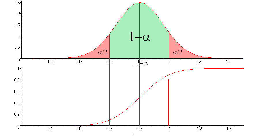
If you choose the level of trust) , the confidence interval is:
, the confidence interval is:
%2B%7B%7B%5CPhi%20%7D%5E%7B-1%7D%7D(%5Calpha%20%2F2)%5Csqrt%7B%5Cfrac%7B(1-%5Calpha%20)%5Calpha%20%7D%7BV%7D%7D%3B(1-%5Calpha%20)-%7B%7B%5CPhi%20%7D%5E%7B-1%7D%7D(%5Calpha%20%2F2)%5Csqrt%7B%5Cfrac%7B(1-%5Calpha%20)%5Calpha%20%7D%7BV%7D%7D%20%5Cright))
In the figure, the confidence interval is the x value below the green area.
Assuming that the original sequences have a uniform distribution, the proportion of the sequences that passed the test with probability must fall into this interval.
If you use the "rule ", The interval will be:
-3%5Csqrt%7B%5Cfrac%7B(1-%5Calpha%20)%5Calpha%20%7D%7BV%7D%7D%3B(1-%5Calpha%20)%2B3%5Csqrt%7B%5Cfrac%7B(1-%5Calpha%20)%5Calpha%20%7D%7BV%7D%7D%20%5Cright))
If the calculated share of the sequences falls within the confidence interval, then the test is considered to be passed.
The above is a description of testing one test at a time. If the battery contains several tests, then the described studies are conducted for each test.
At the exit, a plate is issued, which tests have been passed, and the percentage of tests passed.
In the comments to the articles on Habrahabr there are questions about how these packages receive the final figures. In general, there is nothing difficult - it's just statistics. If the reader is interested in the magic of obtaining these figures, then I ask for a cat, there are a lot of beeches and formulas.
If possible, I want to make the presentation as clear as possible for an unprepared user, so please forgive for some inaccuracies and omitted definitions.
General scheme
Statistical sequence analysis, as a rule, takes place in two stages.
- The first stage can be called preparatory, it is the most time-consuming, here the bulk of calculations are performed.
1.1. With the help of the generator under study, random sequences are formed.
1.2. For each sequence, test statistics is calculated. If the battery of tests works (several tests are carried out at once), then the statistics on the sequence is calculated for each test.
1.3. For each sequence, the probability of significance is calculated.
1.4. The statistics and probabilities of significance obtained are preserved. - At the second stage, the processing of the obtained results is carried out.
2.1. With the help of the consent criteria, hypotheses about the correspondence of distributions of statistics and significance probabilities to hypothetical distributions are checked.
2.2. Determined by the number of sequences that passed the test. Constructed confidence interval for the last value.
2.3. The decision is made whether the test is passed.
2.4. Final conclusions.
Schematically, this process can be represented like this:
')
Formation of statistics
The goal of each test is to test the hypothesis that the sequence under investigation has a uniform distribution. Speaking more strictly, each sign
And from where do the formulas for test statistics appear? Let's take a look at the example of a frequency test from the NIST package.
Each statistical test tests some assumption about a particular property that a random sequence must have that satisfies the hypothesis.
For the frequency test from the NIST test suite, this assumption is the statement: “If the sequence satisfies the hypothesis
If we find the sum of characters of the sequence under study, then the final result will be a random variable, let's call it
Since we are interested in the deviation of the number of units (zeros) from the expectation, we will consider a random variable
The result was a random variable depending on the sequence under study. The distribution function of this random variable under the hypothesis assumption
Where
The value of S calculated for a particular sequence X is called "statistics". If you look at the NIST test descriptions, you can find this particular formula for calculating test statistics.
Using the same reasoning, formulas for other tests appear.
How to distinguish the "good" sequence from the "bad"?
It is necessary to determine whether the statistics S deviates significantly from zero or not.
Deviation should not be "too" big. The word "too" does not give specific instructions for action. Therefore, we choose some critical level
In other words
In packages of statistical studies, another equivalent decision-making method is often used. According to statistics, S calculates the probability of significance p, which is equal to:
Usually
Further conclusions
Immediately the question arises: "How to reject a generator of (pseudo) random numbers, if part of the sequences is bad, and part is good?"
In fact, any random sequence generator will always generate part of the sequences that fail the test. I would even say that if all the sequences pass the test, it is very suspicious.
So, processing the results.
At the first stage, V sequences of length n are generated -
At the second stage, the received samples are processed.
At first, consent criteria are applied to these sequences. Sample
In general, the application of these criteria is similar to the performance of the statistical test described above. The only difference is in the applied statistics.
Application of Pearson's criterion
For
The range of possible values of P (segment [0,1]) is divided by T equal segments. The value of T is usually chosen not very large, for example, 10 or 20. Assuming that P has a uniform distribution, on average, V / T values should fall into each interval (by the way, T should be chosen so that V / T> 5).
Sample P is formed histogram
For statistics
How many sequences must pass the test?
Next, we examine the number of sequences that passed the test.
Since significance probabilities are distributed evenly over the [0,1] interval, on average, the test must pass
Let me give you a confidence interval for the proportion of sequences that passed the test.
Sequences
According to the central limit theorem, the distribution of the number of successes in the Bernoulli test sequence, which coincides with the number of sequences that passed the test, can be considered normal with the expectation
If you choose the level of trust
In the figure, the confidence interval is the x value below the green area.
Assuming that the original sequences have a uniform distribution, the proportion of the sequences that passed the test with probability
If you use the "rule
If the calculated share of the sequences falls within the confidence interval, then the test is considered to be passed.
How the battery of tests works
The above is a description of testing one test at a time. If the battery contains several tests, then the described studies are conducted for each test.
At the exit, a plate is issued, which tests have been passed, and the percentage of tests passed.
Literature
- NIST (statistical test suite for cryptographic applications), http://csrc.nist.gov
- Ivchenko G.I., Medvedev Yu.I. Mathematical Statistics: Textbook. manual for technical colleges. - M .: Higher. shk., 1984.
- Knut D. The art of programming: in 3t. - M .: Mir, 1992
- Van der Warden, BL, Mathematical Statistics. - M .: Publishing house of foreign literature, 1960
Source: https://habr.com/ru/post/276535/
All Articles