Machine learning from Octave \ Matlab to Python

I decided to get acquainted with such an interesting area for me as Machine learning. After a brief search, I found a fairly popular course at Stanford University Machine learning. It tells you the basics and gives a broad overview of machine learning, datamining, and statistical pattern recognition. There was for me a small minus in this course as a Python programmer — homework had to be done on Octave \ Matlab. As a result, I didn’t regret getting a new programming language idea, but as a learning example I decided to rewrite my homework in Python as a learning example for getting closer acquainted with the relevant libraries. What happened is on GitHub here .

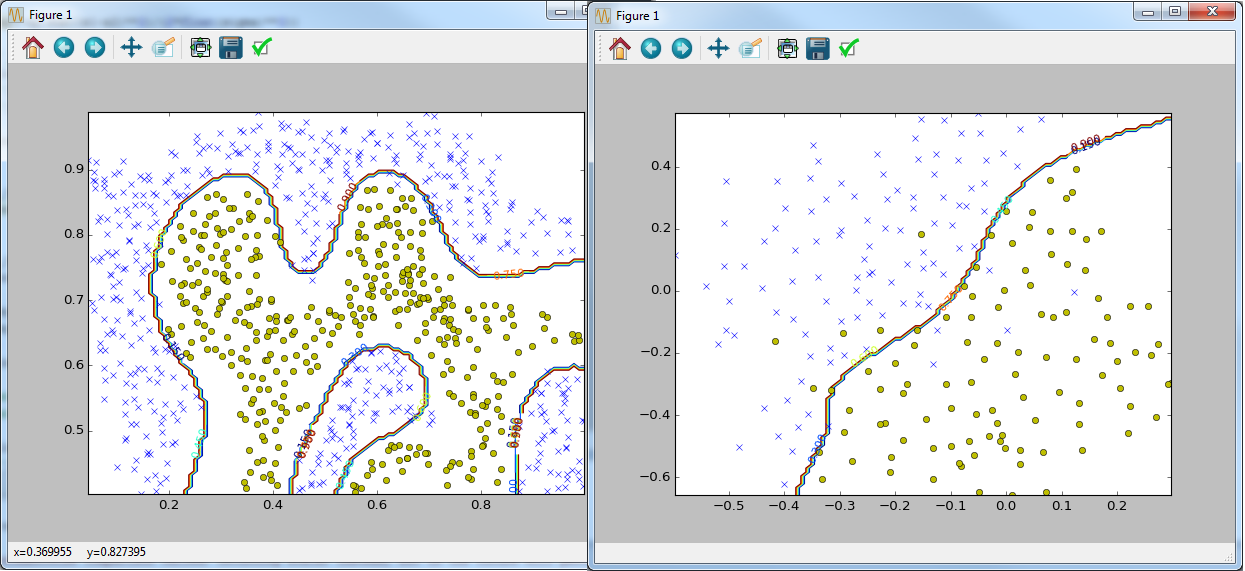
if __name__ == '__main__': data = sio.loadmat('ex6data1.mat') y = data['y'].astype(np.float64) X = data['X'] visualize_boundary_linear(X, y, None) C = 1 model = svm_train(X, y, C, linear_kernel, 0.001, 20) visualize_boundary_linear(X, y, model) C = 100 model = svm_train(X, y, C, linear_kernel, 0.001, 20) visualize_boundary_linear(X, y, model) x1 = np.array([1, 2, 1], dtype=np.float64) x2 = np.array([0, 4, -1], dtype=np.float64) sigma = 2.0 sim = gaussian_kernel(x1, x2, sigma); print('Gaussian Kernel between x1 = [1; 2; 1], x2 = [0; 4; -1], sigma = 0.5 : (this value should be about 0.324652)') print('Actual = {}'.format(sim)) data = sio.loadmat('ex6data2.mat') y = data['y'].astype(np.float64) X = data['X'] visualize_data(X, y).show() C = 1.0 sigma = 0.1 partialGaussianKernel = partial(gaussian_kernel, sigma=sigma) partialGaussianKernel.__name__ = gaussian_kernel.__name__ model= svm_train(X, y, C, partialGaussianKernel) visualize_boundary(X, y, model) data = sio.loadmat('ex6data3.mat') y = data['y'].astype(np.float64) X = data['X'] Xval = data['Xval'] yval = data['yval'].astype(np.float64) visualize_data(X, y).show() best_C = 0 best_sigma = 0 best_error = len(yval) best_model = None for C in [0.01, 0.03, 0.1, 0.3, 1, 3, 10, 30]: for sigma in [0.01, 0.03, 0.1, 0.3, 1, 3, 10, 30]: partialGaussianKernel = partial(gaussian_kernel, sigma=sigma) partialGaussianKernel.__name__ = gaussian_kernel.__name__ model= svm_train(X, y, C, partialGaussianKernel) ypred = svm_predict(model, Xval) error = np.mean(ypred != yval.ravel()) if error < best_error: best_error = error best_C = C best_sigma = sigma best_model = model visualize_boundary(X, y, best_model) 

But since Python has its own popular scikit-learn library for this purpose, I tried to rewrite some tasks using this feature (corresponding files with the suffix sklearn). As expected, the code with the library is fast and looks more compact and clearer (from my point of view).

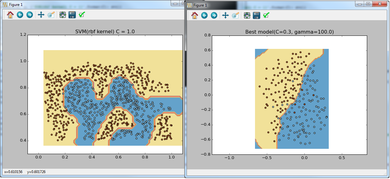
 if __name__ == '__main__': data = sio.loadmat('ex6data1.mat') y = data['y'].astype(np.float64).ravel() X = data['X'] visualize_boundary(X, y, None) C = 1 lsvc = LinearSVC(C=C, tol=0.001) lsvc.fit(X, y) svc = SVC(C=C, tol=0.001, kernel='linear') svc.fit(X, y) visualize_boundary(X, y, {'SVM(linear kernel) C = {}'.format(C): svc, 'LinearSVC C = {}'.format(C): lsvc}) C = 100 lsvc = LinearSVC(C=C, tol=0.001) lsvc.fit(X, y) svc = SVC(C=C, tol=0.001, kernel='linear') svc.fit(X, y) visualize_boundary(X, y, {'SVM(linear kernel) C = {}'.format(C): svc, 'LinearSVC C = {}'.format(C): lsvc}) data = sio.loadmat('ex6data2.mat') y = data['y'].astype(np.float64).ravel() X = data['X'] visualize_boundary(X, y) C = 1.0 sigma = 0.1 gamma = sigma_to_gamma(sigma) svc = SVC(C=C, tol=0.001, kernel='rbf', gamma=gamma) svc.fit(X, y) visualize_boundary(X, y, {'SVM(rbf kernel) C = {}'.format(C): svc}) data = sio.loadmat('ex6data3.mat') y = data['y'].astype(np.float64).ravel() X = data['X'] Xval = data['Xval'] yval = data['yval'].astype(np.float64).ravel() visualize_boundary(X, y) C_coefs = [0.01, 0.03, 0.1, 0.3, 1, 3, 10, 30] sigma_coefs = [0.01, 0.03, 0.1, 0.3, 1, 3, 10, 30] svcs = (SVC(C=C, gamma=sigma_to_gamma(sigma), tol=0.001, kernel='rbf') for C in C_coefs for sigma in sigma_coefs) best_model = max(svcs, key=lambda svc: svc.fit(X, y).score(Xval, yval)) visualize_boundary(X, y, {'Best model(C={}, gamma={})'.format(best_model.C, best_model.gamma): best_model}) #Let's do the similar thing but using sklearn feature X_all = np.vstack((X, Xval)) y_all = np.concatenate((y, yval)) parameters = {'C':C_coefs, 'gamma': map(sigma_to_gamma, sigma_coefs)} svr = SVC(tol=0.001, kernel='rbf') clf = GridSearchCV(svr, parameters, cv=2) clf.fit(X_all, y_all) visualize_boundary(X, y, {'Best model(C={}, gamma={})'.format(clf.best_params_['C'], clf.best_params_['gamma']): clf}) 

')


PS
For those who are interested in the Sklearn library, I would advise:
Udacity course
Video 1 with pycon
Video 2 with pycon

Pps
To develop and run the examples I used the Anaconda distribution.