Adjusted sliding exam, coclassifiers, fractal classifiers and local error probability
This paper presents elements of an introduction to the classification with training on small samples - from a convenient notation to special assessments of reliability. The constant increase in the speed of computing devices and small samples make it possible to neglect the considerable amount of computation needed to obtain some of these estimates.
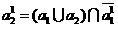
Let some initial partition of the set be given of objects
  into two subsets (classes)
  such that
 ,
,  .
.
(one)
We will identify a two-class classifier with a binary function of the form

(2)
Where - random sampling subsets
 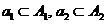 from classes , -examined object that must be attributed to one of the classes. The values of this function will be interpreted as “solutions” in accordance with the rule
(3)
')
Depending on whether or not the solutions of the classifier correspond to the original partition into classes, we will consider them respectively “correct” or “erroneous”. We also agree  elements of samples denote
  so that respectively:
 ,
,
(four)
Where - the volume of training samples. Set a lot "Immersed" in
  -dimensional right-side Euclidean space
  . Then all the elements of the classes , including, of course, the elements of the training samples and the object under study can be regarded as its points. Coordinates of point features from the set we will mark the right subscript
  . Object coordinates
  training samples will be written as
  object under study as -
  . Depending on the context, understood either as an object name or as a radius vector.
We proceed from the absence of a test sequence, and the estimation of the probability of a classification error feasible in a sliding exam
 ,
,
(five)
Where
 ,
,
(6)
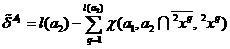 .
.
(7)
Objects the training samples classified in the sliding exam mode will be called quasi-replaceable in the future.
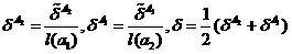
Sliding exam, as you know, has several drawbacks. These deficiencies can be eliminated to some extent through the correction of the sliding exam. The adjusted scores marked with the left stroke will be written as follows.
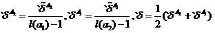 ,
,
(eight)
 ,
,
(9)
 .
.
(ten)
The disadvantages of the adjusted sliding exam include the increase in the number of operations and the fact that this assessment is carried out on both samples per unit of smaller volume. Thus, for small samples, the estimate of the error probability is somewhat overestimated, however, with an increase in the sample size, this effect loses its value.
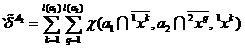
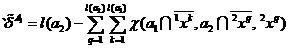
Due to the large laboriousness of the corrected sliding exam, the method of binary assessment of the reliability of the classification - classifier is of interest. Like the sliding exam, it can be based solely on information from training samples, but it can also be used if there are test sequences.
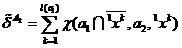
Let's enter selections objects, respectively, correctly and erroneously classified by the classifier (2) in the sliding exam mode
 ,
,
(eleven)
 .
.
(12)
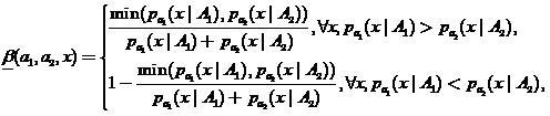
Then the solution of the coclassifier of the first order classifier (2), defined as
 ,
,
(13)
interpreted as follows
if a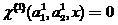 then the classifier (2) made the right decision regarding ,
if a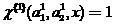 then the classifier (2) made the wrong decision regarding .
(14)
In this case, we assume that the sample extracted from certain classes
  objects, potentially correctly or mistakenly referred by the classifier (2).
In determining (13), it is assumed that the sample size not too small. Thus, if we only have the material of training samples, and there are no check sequences, then it is recommended to use a coclassifier in conditions when the classifier (2) makes a significant amount of errors. If you still use the co-classifier in a small sample then it should be chosen in a fairly simple form. For example, if the co-classifier is of the Fisher type, one can assume the diagonality of the covariance matrix or even its singularity.
Like adaptive boosting, classifier composition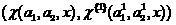 can be considered as a collective classifier, organized much more nonlinearly compared to those proposed in [1].
Let us dwell on issues related to the choice of a particular form of co-classifier. Let, for example, the sample extracted from classes with density of distributions  and the classes overlap a lot. In this case, it can often turn out that the sample density
  have close mean values. In this case, the co-classifier can be chosen, for example, in the form of a linear Fisher classifier modified using the Peterson-Mattson procedure [2,3].
The process of synthesis of co-classifiers of higher orders can be continued in the framework of the recurrent procedure, when the initial substitution is performed
 ,
,
(15)
then, repeating the above algorithm, we get the second-order co-classifier at the output
 .
.
(sixteen)
and continue this procedure. An imperative stop occurs when building a co-classifier of this order. in which
  or even
  . As a result, we obtain an iterated classifier system — the fractal classifier. This collective classifier should not, of course, be confused with image classifiers using fractal and wavelet transformations to process them.
In practice, we had to use only co-classifiers of the first order. They were developed by us many years ago and have proven to be useful tools in solving various practical problems, in particular, in the analysis of reflected radio signals for installations searching for anti-personnel plastic mines [4], as well as in creating the LEKTON system. This system made it possible to fully automatically verify the authenticity of signatures on checks, bills and other documents and was the first system of this type actually used at the bank.
In practical studies, local ones have proven themselves well. - estimates of the probability of classification error. Let the classifier (2) be in the form
 ,
,
(17)
Where - density estimates by samples respectively. Then local - the estimate of the probability of error of this classifier can be defined as
 ,
,
(18)
Where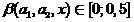 .
.
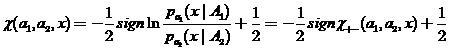
We introduce a special - assessment, which can be considered as a “blurred” classifier
(nineteen)
Where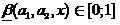 . Then we will assume that
  interpreted as a blurry classifier solution that
  ,
, 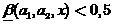 - as a decision that
  . At the same time, the closer
  to zero or to one, the corresponding decisions of the fuzzy classifier are more trustworthy.
Based on the estimate (19), one can summarize the definition of the classifier (2) by entering the zone of failure or zone of failure. Denoting the width of these zones respectively , we will present them in the following form
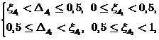
(20)
Where - boundaries of zones. In the absence of asymmetry in the requirements for zones is selected
  .
.
Literature:
1. Archipov GF Collectives of determinative rules: - In the Collection of articles “Statistical problems of control”, Vilnius, 1983, vol.61, pp. 130-145.
2. Myasnikov V.V. Modifications of the method for constructing a linear discriminant function based on the Peterson-Mattson procedure. computeroptics.smr.ru/KO/PDF/KO26/KO26211.pdf.
3. Fukunaga K. Introduction to the statistical theory of pattern recognition. M. "Science" 1979. pp. 105-130.
4. Archipov, G., Klyshko, G., Stasaitis, D., Levitas, B., Alenkowicz, H., Jefremov, S.C. MIKON-2000., XII International Conference on Microwaves, Radar and Wireless Communications, Volume 2, pp. 495-498 ./>
Definitions and designations
Let some initial partition of the set be given
of objects into two subsets (classes) such that , .(one)
We will identify a two-class classifier with a binary function of the form
(2)
Where
- random sampling subsets from classes , -examined object that must be attributed to one of the classes. The values of this function will be interpreted as “solutions” in accordance with the rule(3)
')
Depending on whether or not the solutions of the classifier correspond to the original partition
into classes, we will consider them respectively “correct” or “erroneous”. We also agree elements of samples denote so that respectively: ,(four)
Where
- the volume of training samples. Set a lot "Immersed" in -dimensional right-side Euclidean space . Then all the elements of the classes , including, of course, the elements of the training samples and the object under study can be regarded as its points. Coordinates of point features from the set we will mark the right subscript . Object coordinates training samples will be written as object under study as - . Depending on the context, understood either as an object name or as a radius vector.We proceed from the absence of a test sequence, and the estimation of the probability of a classification error
feasible in a sliding exam ,(five)
Where
,(6)
.(7)
Objects
the training samples classified in the sliding exam mode will be called quasi-replaceable in the future.Adjusted sliding exam
Sliding exam, as you know, has several drawbacks. These deficiencies can be eliminated to some extent through the correction of the sliding exam. The adjusted scores marked with the left stroke will be written as follows.
,(eight)
,(9)
.(ten)
The disadvantages of the adjusted sliding exam include the increase in the number of operations and the fact that this assessment is carried out on both samples per unit of smaller volume. Thus, for small samples, the estimate of the error probability is somewhat overestimated, however, with an increase in the sample size, this effect loses its value.
Classifier
Due to the large laboriousness of the corrected sliding exam, the method of binary assessment of the reliability of the classification - classifier is of interest. Like the sliding exam, it can be based solely on information from training samples, but it can also be used if there are test sequences.
Let's enter selections
objects, respectively, correctly and erroneously classified by the classifier (2) in the sliding exam mode ,(eleven)
.(12)
Then the solution of the coclassifier of the first order classifier (2), defined as
,(13)
interpreted as follows
if a
then the classifier (2) made the right decision regarding ,if a
then the classifier (2) made the wrong decision regarding .(14)
In this case, we assume that the sample
extracted from certain classes objects, potentially correctly or mistakenly referred by the classifier (2).In determining (13), it is assumed that the sample size
not too small. Thus, if we only have the material of training samples, and there are no check sequences, then it is recommended to use a coclassifier in conditions when the classifier (2) makes a significant amount of errors. If you still use the co-classifier in a small sample then it should be chosen in a fairly simple form. For example, if the co-classifier is of the Fisher type, one can assume the diagonality of the covariance matrix or even its singularity.Like adaptive boosting, classifier composition
can be considered as a collective classifier, organized much more nonlinearly compared to those proposed in [1].Let us dwell on issues related to the choice of a particular form of co-classifier. Let, for example, the sample
extracted from classes with density of distributions and the classes overlap a lot. In this case, it can often turn out that the sample density have close mean values. In this case, the co-classifier can be chosen, for example, in the form of a linear Fisher classifier modified using the Peterson-Mattson procedure [2,3].Fractal classifier
The process of synthesis of co-classifiers of higher orders can be continued in the framework of the recurrent procedure, when the initial substitution is performed
,(15)
then, repeating the above algorithm, we get the second-order co-classifier at the output
.(sixteen)
and continue this procedure. An imperative stop occurs when building a co-classifier of this order.
in which or even . As a result, we obtain an iterated classifier system — the fractal classifier. This collective classifier should not, of course, be confused with image classifiers using fractal and wavelet transformations to process them.In practice, we had to use only co-classifiers of the first order. They were developed by us many years ago and have proven to be useful tools in solving various practical problems, in particular, in the analysis of reflected radio signals for installations searching for anti-personnel plastic mines [4], as well as in creating the LEKTON system. This system made it possible to fully automatically verify the authenticity of signatures on checks, bills and other documents and was the first system of this type actually used at the bank.
Local error probability
In practical studies, local ones have proven themselves well.
- estimates of the probability of classification error. Let the classifier (2) be in the form ,(17)
Where
- density estimates by samples respectively. Then local - the estimate of the probability of error of this classifier can be defined as ,(18)
Where
.We introduce a special
- assessment, which can be considered as a “blurred” classifier(nineteen)
Where
. Then we will assume that interpreted as a blurry classifier solution that , - as a decision that . At the same time, the closer to zero or to one, the corresponding decisions of the fuzzy classifier are more trustworthy.Based on the estimate (19), one can summarize the definition of the classifier (2) by entering the zone of failure or zone of failure. Denoting the width of these zones respectively
, we will present them in the following form(20)
Where
- boundaries of zones. In the absence of asymmetry in the requirements for zones is selected .Literature:
1. Archipov GF Collectives of determinative rules: - In the Collection of articles “Statistical problems of control”, Vilnius, 1983, vol.61, pp. 130-145.
2. Myasnikov V.V. Modifications of the method for constructing a linear discriminant function based on the Peterson-Mattson procedure. computeroptics.smr.ru/KO/PDF/KO26/KO26211.pdf.
3. Fukunaga K. Introduction to the statistical theory of pattern recognition. M. "Science" 1979. pp. 105-130.
4. Archipov, G., Klyshko, G., Stasaitis, D., Levitas, B., Alenkowicz, H., Jefremov, S.C. MIKON-2000., XII International Conference on Microwaves, Radar and Wireless Communications, Volume 2, pp. 495-498 ./>
Source: https://habr.com/ru/post/276017/
All Articles