Python and beautiful legs: how I would introduce my son to mathematics and programming
Previously, we were already looking for unusual Playboy models using the Python Scikit-learn library. Now we will demonstrate some of the capabilities of the SymPy, SciPy, Matplotlib and Pandas libraries using a living example from the category of entertaining school math problems. The goal is to ease the threshold for examining Python libraries for analyzing data.

')
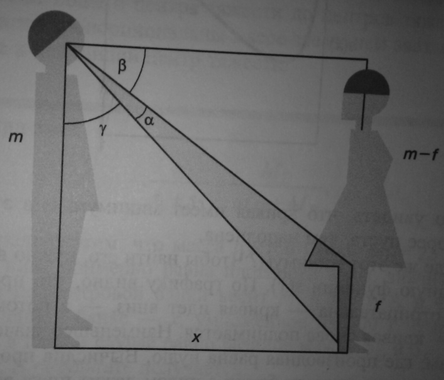
There is a girl with graceful, trained, and most importantly, bare legs. Is bored. Before you demonstrate your (n + 1) level of proficiency in pickup equipment, you want to get a better look at the legs of a girl - is it worth it? Better to look at is at the greatest angle. You can quietly approach the girl (like looking into the distance), but you can not squat - it is necessary as a matter of fact and respect for decency. From what distance are the legs visible at the greatest angle? Suppose your height is such that the eyes are at a height m above the ground. The legs of the girl are bare to a height of f.
Picture and rephrased problem from Christophe Dresser: Seduce with Math. Numeric games for all occasions. Binomial. Laboratory of knowledge, 2015 "
We explain the problem. From a distance, it is difficult to treat the legs - they are visible at a too small angle. But if you get too close, your legs will also be visible at a small angle. Somewhere there should be an optimal distance.
Let x be the distance to the girl, f is the length of the bare part of the girl's legs, alpha is the angle at which the legs are visible (must be maximized).
The alpha angle is easiest to find by subtracting the angles beta and gamma from a right angle. If school trigonometry is still somehow alive in the back streets of the brain, it’s easy to get that
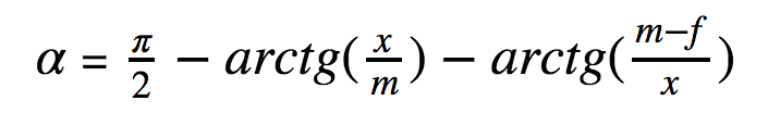
The task is to maximize alpha (x) with respect to the variable x.
Well, this is also simple, we say: we zero the derivative - and go!
To begin with, we construct a graph of the function alpha (x). For definiteness, we take the values of the parameters m = 1.7 m and f = 0.7 m (I would like 1 m, but still it is assumed that there is some skirt).
Now the code. Anaconda assembly and IPython notebooks are used. The code is reproducible, lies in the GitHub repository .
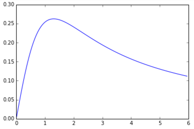
ABOUT! The assumption was confirmed: somewhere in the 1-1.5 m from the girl her legs are visible at the greatest angle. Well ... it's hard without pale. Let's now find the exact value of the optimal distance to the girl.
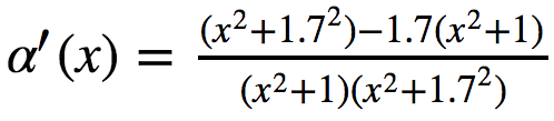
The analytical solution is very simple; it suffices to remember the derivative of the arctangent. On Habré, LaTeX is not supported, so this part is in the corresponding IPython notebook.
The result is:

SymPy is a Python symbol computing library. We will look at how to use it to calculate derivatives (the diff method) and find the roots of the equations (the solve method).
Let's get the character variable x and the function alpha (x). For symbolic calculations, the number Pi and the arctangent must also be taken from SymPy.
Calculate the derivative of alpha '(x). The diff method must specify the function, the variable by which differentiation occurs, and the order of the derivative, in this case 1.
You can make sure that this is the same thing that worked, if you pick up a pencil and paper.
As you can see, SymPy simply does not lead to a common denominator. There is a simplify method for this.
Now find the zeros of the derivative using the solve method.
Again, we got that it’s best to look at a girl from about 1.3 meters. Interestingly, do photographers also do such calculations?
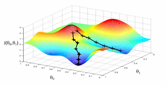
Picture from Andrew Ng machine learning course
In addition to everything useful, the SciPy library implements various methods of numerical optimization. For a detailed description of many methods for minimizing one-dimensional and multi-dimensional functions, see the documentation for the scipy.optimize.minimize method.
There is no maximize method per se, so the maximization problem will be emulated by minimizing the function multiplied by (-1). Consider the simplest case - the minimization of the scalar function of one variable. The optimization methods of 'brent', 'bounded' and 'golden' have been implemented, but for some reason the differences have not been properly documented .
The answer is the same as expected.
Now we will choose a girl whose legs we will admire. Let's return to the familiar girls.csv data set by Playboy models of the month. Choose the highest of non-dystrophic girls. At the same time we will show something from the Pandas library.
To find among the Playboy models a girl with the highest height with a “normal” body mass index - from 18 to 18.5.
Create a new sign BMI - body mass index , equal to weight divided by height in meters squared.
Construct a BMI distribution histogram.

Wikipedia says that the normal BMI is 18.5–24.99. We see that the average index for Playboy models is approximately at the lower limit of the norm.
We will select girls with a BMI of 18 to 18.5.
This is the July July 1994 version of Playboy Traci Adell. Further search engine to help. This choice is unlikely to disappoint.
So, we looked at the very basics of using the Python SymPy, SciPy and Pandas libraries. An abundance of examples of the actual use of these libraries can be found in the GitHub repositories. One of the reviews of such repositories here .
')
Task 1
There is a girl with graceful, trained, and most importantly, bare legs. Is bored. Before you demonstrate your (n + 1) level of proficiency in pickup equipment, you want to get a better look at the legs of a girl - is it worth it? Better to look at is at the greatest angle. You can quietly approach the girl (like looking into the distance), but you can not squat - it is necessary as a matter of fact and respect for decency. From what distance are the legs visible at the greatest angle? Suppose your height is such that the eyes are at a height m above the ground. The legs of the girl are bare to a height of f.
Decision
Picture and rephrased problem from Christophe Dresser: Seduce with Math. Numeric games for all occasions. Binomial. Laboratory of knowledge, 2015 "
We explain the problem. From a distance, it is difficult to treat the legs - they are visible at a too small angle. But if you get too close, your legs will also be visible at a small angle. Somewhere there should be an optimal distance.
Let x be the distance to the girl, f is the length of the bare part of the girl's legs, alpha is the angle at which the legs are visible (must be maximized).
The alpha angle is easiest to find by subtracting the angles beta and gamma from a right angle. If school trigonometry is still somehow alive in the back streets of the brain, it’s easy to get that
The task is to maximize alpha (x) with respect to the variable x.
Well, this is also simple, we say: we zero the derivative - and go!
To begin with, we construct a graph of the function alpha (x). For definiteness, we take the values of the parameters m = 1.7 m and f = 0.7 m (I would like 1 m, but still it is assumed that there is some skirt).
Now the code. Anaconda assembly and IPython notebooks are used. The code is reproducible, lies in the GitHub repository .
# Anaconda import warnings warnings.filterwarnings('ignore') # IPython, %pylab inline import numpy as np from math import pi, atan def alpha(x, m, f): return pi/2 - atan(x/m) - atan((mf)/x) # x = np.arange(0, 6, 0.05) plot(x, [alpha(i, 1.7, 0.7) for i in x]) ABOUT! The assumption was confirmed: somewhere in the 1-1.5 m from the girl her legs are visible at the greatest angle. Well ... it's hard without pale. Let's now find the exact value of the optimal distance to the girl.
Analytical solution "by hand"
The analytical solution is very simple; it suffices to remember the derivative of the arctangent. On Habré, LaTeX is not supported, so this part is in the corresponding IPython notebook.
The result is:
Analytical solution with SymPy
SymPy is a Python symbol computing library. We will look at how to use it to calculate derivatives (the diff method) and find the roots of the equations (the solve method).
import sympy as sym Let's get the character variable x and the function alpha (x). For symbolic calculations, the number Pi and the arctangent must also be taken from SymPy.
x = sym.Symbol('x') alpha = sym.pi/2 - sym.atan(x/1.7) - sym.atan(1/x) alpha # -atan(1/x) - atan(0.588235294117647*x) + pi/2 Calculate the derivative of alpha '(x). The diff method must specify the function, the variable by which differentiation occurs, and the order of the derivative, in this case 1.
alpha_deriv = sym.diff(alpha, x, 1) alpha_deriv # -0.59/(0.35*x**2 + 1) + 1/(x**2*(1 + x**(-2))) You can make sure that this is the same thing that worked, if you pick up a pencil and paper.
As you can see, SymPy simply does not lead to a common denominator. There is a simplify method for this.
sym.simplify(alpha_deriv) # (-0.24*x**2 + 0.41)/((0.35*x**2 + 1)*(x**2 + 1)) Now find the zeros of the derivative using the solve method.
sym.solve(alpha_deriv, x) # [-1.30384048104053, 1.30384048104053] Again, we got that it’s best to look at a girl from about 1.3 meters. Interestingly, do photographers also do such calculations?
Numerical solution with SciPy
Picture from Andrew Ng machine learning course
In addition to everything useful, the SciPy library implements various methods of numerical optimization. For a detailed description of many methods for minimizing one-dimensional and multi-dimensional functions, see the documentation for the scipy.optimize.minimize method.
There is no maximize method per se, so the maximization problem will be emulated by minimizing the function multiplied by (-1). Consider the simplest case - the minimization of the scalar function of one variable. The optimization methods of 'brent', 'bounded' and 'golden' have been implemented, but for some reason the differences have not been properly documented .
from scipy.optimize import minimize_scalar alpha = lambda x: -(pi/2 - atan(x/1.7) - atan(1/x)) result = minimize_scalar(alpha, bounds=[0., 100.], method = 'bounded') The answer is the same as expected.
result.x # 1.3038404104038319 Now we will choose a girl whose legs we will admire. Let's return to the familiar girls.csv data set by Playboy models of the month. Choose the highest of non-dystrophic girls. At the same time we will show something from the Pandas library.
Task 2
To find among the Playboy models a girl with the highest height with a “normal” body mass index - from 18 to 18.5.
Decision
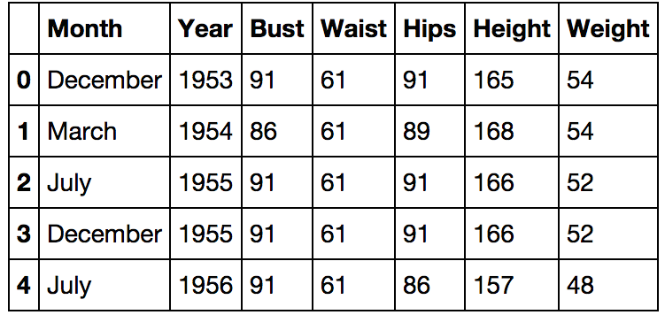
import pandas as pd girls = pd.read_csv('girls.csv') # Pandas.DataFrame girls.head() # 5 Create a new sign BMI - body mass index , equal to weight divided by height in meters squared.
girls['BMI'] = 100 ** 2 * girls['Weight'] / (girls['Height'] ** 2) Construct a BMI distribution histogram.
girls['BMI'].hist() Wikipedia says that the normal BMI is 18.5–24.99. We see that the average index for Playboy models is approximately at the lower limit of the norm.
We will select girls with a BMI of 18 to 18.5.
selected_girls = girls[(girls['BMI'] >= 18) & (girls['BMI'] <= 18.5)] selected_girls.sort(columns=['Height', 'Bust'], ascending=[False, False]).head(1) # Month Year Bust Waist Hips Height Weight BMI #430 July 1994 91 61 91 180 59 18.209877 This is the July July 1994 version of Playboy Traci Adell. Further search engine to help. This choice is unlikely to disappoint.
So, we looked at the very basics of using the Python SymPy, SciPy and Pandas libraries. An abundance of examples of the actual use of these libraries can be found in the GitHub repositories. One of the reviews of such repositories here .
Source: https://habr.com/ru/post/275963/
All Articles