Considering difference schemes in Mathcad Express
I continue sketching about using the free math editor Mathcad Express . This time, I propose to turn to the numerical solution of differential equations (in today's example, with partial derivatives). You can find the file with further calculations in Mathcad and XPS formats here .
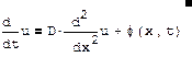
In this article, we consider how to calculate the differential equation of heat diffusion using the simplest explicit difference scheme in Mathcad Express and dwell on the stability property of difference schemes. It will be discussed how to get this solution to the equation that simulates the cooling of a one-dimensional object:

')
The graph shows the initial temperature distribution along the X axis (red line) and two calculated profiles after the first step and after several time steps.
As an example of a partial differential equation, we consider the heat equation (or, alternatively, heat diffusion).
This equation is of parabolic type, containing the first derivative with respect to time t and the second with respect to the spatial coordinate x. It describes the dynamics of temperature u (x, t) in the presence of heat sources, for example, when a metal rod is heated. Thus, the unknown function to be defined is the function u (x, t). This equation is linear if the source and diffusion coefficient D are either independent of temperature or the source depends linearly on it, since in this case, the unknown function u (x, t) (and all its derivatives) enters the equation in the first degree.
The linear heat equation has an analytical solution, while the vast majority of nonlinear partial differential equations can only be solved numerically. In order for partial differential equations to have a unique solution, it is necessary to set the required number of initial and boundary conditions, i.e., in this case, relations of the type u (x, 0) = Init (x) (initial condition) together with u (0, t) = f1 (t) and u (L, t) = f2 (t) (boundary conditions if the equation is solved in the interval from 0 to L).
In the above interpretation, the one-dimensional heat diffusion equation describes the temperature dynamics of some elongated body, for example, a metal rod:

We will consider the case of a zero heat source, and as the initial condition we choose some realistic temperature profile (the rod is very hot in the center). As the boundary conditions, we set the maintenance of the edges of the rod at a constant temperature. Of course, the solution dynamics describes the expected pattern of rod temperature equalization with time (due to heat transfer from the center to the periphery of the rod due to the heat conduction mechanism). The heat transfer rate is determined by the value of the diffusion coefficient D. (For the interested reader, I suggest experimenting with the calculations in Mathcad Express, choosing different values of the diffusion coefficient).
We show how to implement in Mathcad the main computational approach to solving partial differential equations - the grid method. We will do it "manually" in order not to go beyond the free version of Mathcad Express.
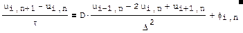
The essence of the grid method is to cover the computational domain (x, t) with a grid of MxN points, which will determine the steps in time and space τ and Δ, respectively. Thereby, the nodes in which the solution will be searched are determined. Then it is necessary to replace the differential equation with an approximating equation of it in finite differences, for each (i, n) -th grid node. In the case of the heat equation, it is sufficient to simply replace the first derivative with respect to time and the second in space with their difference analogues (this discretization method is called the Euler method, and the resulting system of difference equations with a difference scheme).
The written scheme is explicit, since in it, the unknown value of the desired function (at the n + 1 time step) can be expressed in terms of the previously calculated function values at the previous nth step (“layer”) over time. Moreover, since and on each stratum the equations are interconnected recurrently, i.e. the value in each unknown node on the nth layer can be found, knowing only the previously calculated values from the previous layer. This allows you to organize a process so-called. “Running account”, solving the corresponding equations on each layer (based on the known solution on the previous layer).
The following calculation implements the described algorithm of the explicit explicit scheme of a running account in Mathcad Express:

Actually, the calculated values of the matrix U are shown in the graph, which was shown at the very beginning of the article (before kata).
In conclusion, we dwell on the stability property of difference schemes. The task parameter that characterizes the ratio of the steps of the difference scheme in space and time is called the Courant coefficient (or "number"):

It is significant that the previous calculations according to an explicit scheme were carried out with the Courant ratio less than 1. But if you try to increase the time step in the explicit scheme, so that the Courant ratio becomes more than 1, then we will encounter a catastrophe: the solution “collapses”, and instead of the expected (and calculated at smaller Courant ratios for cases) the solution results in a rapidly oscillating, totally implausible solution.

This example demonstrates an important property of difference schemes, called stability. It turns out that many schemes (of course, or at a certain ratio of parameters, like our scheme) do not possess them, and such schemes cannot be used to solve problems.
For more information on difference schemes and examples of their calculation in Mathcad, the reader can find in my book on computational physics (chapters 5 and 6 are devoted to difference schemes, the book is freely available). In particular, I propose to try to solve the difference method "inverse heat conduction equation", which is obtained by replacing the variable t with -t and which (in theory) should describe the reconstruction of the initial temperature profile of the rod according to the observation after some time.
And I repeat that the file with the calculations described in this article can be found here , and the Mathcad Express distribution can be downloaded here .
In this article, we consider how to calculate the differential equation of heat diffusion using the simplest explicit difference scheme in Mathcad Express and dwell on the stability property of difference schemes. It will be discussed how to get this solution to the equation that simulates the cooling of a one-dimensional object:
')
The graph shows the initial temperature distribution along the X axis (red line) and two calculated profiles after the first step and after several time steps.
Heat equation
As an example of a partial differential equation, we consider the heat equation (or, alternatively, heat diffusion).
This equation is of parabolic type, containing the first derivative with respect to time t and the second with respect to the spatial coordinate x. It describes the dynamics of temperature u (x, t) in the presence of heat sources, for example, when a metal rod is heated. Thus, the unknown function to be defined is the function u (x, t). This equation is linear if the source and diffusion coefficient D are either independent of temperature or the source depends linearly on it, since in this case, the unknown function u (x, t) (and all its derivatives) enters the equation in the first degree.
The linear heat equation has an analytical solution, while the vast majority of nonlinear partial differential equations can only be solved numerically. In order for partial differential equations to have a unique solution, it is necessary to set the required number of initial and boundary conditions, i.e., in this case, relations of the type u (x, 0) = Init (x) (initial condition) together with u (0, t) = f1 (t) and u (L, t) = f2 (t) (boundary conditions if the equation is solved in the interval from 0 to L).
In the above interpretation, the one-dimensional heat diffusion equation describes the temperature dynamics of some elongated body, for example, a metal rod:
We will consider the case of a zero heat source, and as the initial condition we choose some realistic temperature profile (the rod is very hot in the center). As the boundary conditions, we set the maintenance of the edges of the rod at a constant temperature. Of course, the solution dynamics describes the expected pattern of rod temperature equalization with time (due to heat transfer from the center to the periphery of the rod due to the heat conduction mechanism). The heat transfer rate is determined by the value of the diffusion coefficient D. (For the interested reader, I suggest experimenting with the calculations in Mathcad Express, choosing different values of the diffusion coefficient).
Difference scheme
We show how to implement in Mathcad the main computational approach to solving partial differential equations - the grid method. We will do it "manually" in order not to go beyond the free version of Mathcad Express.
The essence of the grid method is to cover the computational domain (x, t) with a grid of MxN points, which will determine the steps in time and space τ and Δ, respectively. Thereby, the nodes in which the solution will be searched are determined. Then it is necessary to replace the differential equation with an approximating equation of it in finite differences, for each (i, n) -th grid node. In the case of the heat equation, it is sufficient to simply replace the first derivative with respect to time and the second in space with their difference analogues (this discretization method is called the Euler method, and the resulting system of difference equations with a difference scheme).
The written scheme is explicit, since in it, the unknown value of the desired function (at the n + 1 time step) can be expressed in terms of the previously calculated function values at the previous nth step (“layer”) over time. Moreover, since and on each stratum the equations are interconnected recurrently, i.e. the value in each unknown node on the nth layer can be found, knowing only the previously calculated values from the previous layer. This allows you to organize a process so-called. “Running account”, solving the corresponding equations on each layer (based on the known solution on the previous layer).
The following calculation implements the described algorithm of the explicit explicit scheme of a running account in Mathcad Express:
Actually, the calculated values of the matrix U are shown in the graph, which was shown at the very beginning of the article (before kata).
Resilience
In conclusion, we dwell on the stability property of difference schemes. The task parameter that characterizes the ratio of the steps of the difference scheme in space and time is called the Courant coefficient (or "number"):
It is significant that the previous calculations according to an explicit scheme were carried out with the Courant ratio less than 1. But if you try to increase the time step in the explicit scheme, so that the Courant ratio becomes more than 1, then we will encounter a catastrophe: the solution “collapses”, and instead of the expected (and calculated at smaller Courant ratios for cases) the solution results in a rapidly oscillating, totally implausible solution.
This example demonstrates an important property of difference schemes, called stability. It turns out that many schemes (of course, or at a certain ratio of parameters, like our scheme) do not possess them, and such schemes cannot be used to solve problems.
For more information on difference schemes and examples of their calculation in Mathcad, the reader can find in my book on computational physics (chapters 5 and 6 are devoted to difference schemes, the book is freely available). In particular, I propose to try to solve the difference method "inverse heat conduction equation", which is obtained by replacing the variable t with -t and which (in theory) should describe the reconstruction of the initial temperature profile of the rod according to the observation after some time.
And I repeat that the file with the calculations described in this article can be found here , and the Mathcad Express distribution can be downloaded here .
Source: https://habr.com/ru/post/275765/
All Articles