You never would have thought, but this is a walk through the space of a neural network-counterfeiter. Made by the coolest people Anders Boesen Lindbo Larsen and Søren Kaae Sønderby

Suppose we have a task - to understand the world around us.
Let's imagine for simplicity that the world is money.

A metaphor, perhaps with some moral ambiguity, but on the whole the example is not worse than the others - money (banknotes) definitely has some complicated structure, here they have a number, a letter, and there are cunning watermarks. Suppose we need to understand how they are made, and find out the rule by which they are printed. What is the plan?
')
The promising step is to go to the central bank office and ask them to issue a specification, but first, they will not give it to you, and second, if you withstand the metaphor, the universe does not have a central bank (although there are religious differences on this score).

Well, if so, let's try to fake them.

Disriminative vs generative

In general, on the subject of understanding the world there is one fairly well-known approach, which is that to understand is to recognize . That is, when you and I are engaged in some kind of activity in the outside world, we learn to distinguish some objects from others and use them afterwards accordingly. This is a chair, it is sitting on it, and this is an apple, and it is eaten. By consistently observing the required number of chairs and apples, we learn to distinguish them from each other according to the teacher’s instructions, and in this way we discover some heterogeneity and structure in the world.
This is a rather large number of models that we call discriminative . If you are a bit machine-oriented, then you can get into the discriminative model by pointing your finger at random anywhere - multi-layer perceptrons, decisive trees and forests, SVM, you name it. Their task is to assign the correct label to the observed data, and all of them answer the question “what does what I see look like?”

Another approach, slightly completely different, is that to understand is to repeat . That is, if you watched the world for some time, and then you were able to reconstruct a part of it (lay down a paper airplane, for example), then you understood something about how it works. Models that do this usually do not need teacher instructions, and we call them generators - these are all kinds of hidden Markov, naive (and not naive) Bayesian ones, and the modern world of deep neural networks has recently added restricted Boltzmann machines and auto-encoders.

The fundamental difference in these two things is this: in order to recreate a thing, you should know more or less everything about it, but in order to learn how to distinguish one thing from another, it is completely unnecessary. It is best illustrated with this picture:



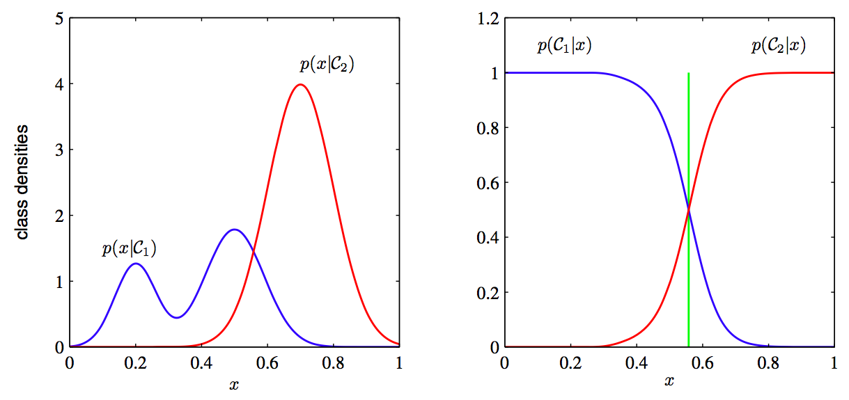
On the left, what the generating model sees (the blue distribution has a complex bimodal structure, and the red one is more narrowed), and on the right, what the discriminative sees (only the border on which the dividing line between the two distributions passes, and she has no idea about the other structure ). A discriminative model sees the world worse - it may well conclude that apples differ from chairs only in that they are red, and this is enough for its purposes.

Both models have their advantages and disadvantages, but for the time being, let's agree for our purpose that the generating model is simply steeper. We like the idea of ​​understanding things completely, not pairwise, comparatively.

How do we generate

Well, well, how do we set up this generating model? For some limited cases, we can use just the theory of probability and the Bayes theorem — say, we are trying to model coin tosses, and assume that they correspond to the binomial distribution, then 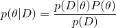and so on. For really interesting objects like pictures or music, this does not work very well - the curse of dimension makes itself felt, there are too many signs (and they depend on each other, so you have to build a joint distribution ...).

A more abstract (and interesting) alternative is to assume that the thing we are modeling can be represented as a small number of hidden variables or "factors." For our hypothetical case of money, this assumption seems to be quite intuitively correct - the drawing on the bill can be decomposed into components in the form of a nominal, serial number, a beautiful picture, an inscription. Then we can say that our source data can be compressed to the size of these factors and restored back without losing the semantic content. On this principle, all kinds of avtoenkodery trying to compress the data and then build their most accurate reconstruction - a very interesting thing, about which we, however, will not speak.

Another method suggested by Ian Goodfellow from Google, and it is this:

1) We create two models, one - generating (let's call it a counterfeiter), and the second - discriminative (let it be a banker)
2) The counterfeiter is trying to build a fake for real money at the exit, and the banker is trying to distinguish the fake from the original (both models start with random conditions and at first give out noise and trash as results).
3) The counterfeiter’s goal is to make a product that a banker could not distinguish from a real one. The goal of the banker is to distinguish counterfeit from the originals as effectively as possible. Both models start the game against each other, where only one will remain .

Both models will be neural networks - hence the name adversarial networks. The article states that the game eventually converges to the victory of a counterfeiter and, accordingly, the defeat of the banker. Good news for the underworld of generative models.

Little formalism

Let's call our counterfeiter (or generator), and banker - (or discriminator). We have some amount of original money. for a banker, and let him have a number from zero to one at the exit, so that it expresses the banker's confidence that the money given to him for consideration is real. Also, since the counterfeiter has a neural network, it needs some input data, let's call it . In fact, this is just a random noise that the model will try to turn into money.

Then, obviously, the counterfeiter’s goal is to maximize , that is, to make so that the banker was sure that the fakes are real.

The banker's goal is more complicated - he needs to simultaneously positively recognize the originals, and negatively - fakes. We write this as maximization 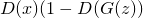. Multiplication can be turned into addition if we take the logarithm, so we get:

For a banker: maximize
For counterfeiter: maximize

This is a little less than all the math that we need here.

One dimensional example

(almost entirely taken from this wonderful post , but there - on TensorFlow)

Let's try to solve a simple one-dimensional example: let our models deal with ordinary numbers that have condensed around a point. on a small scale . The probability of each met number found somewhere on the number line can be represented by a normal distribution. Here it is:



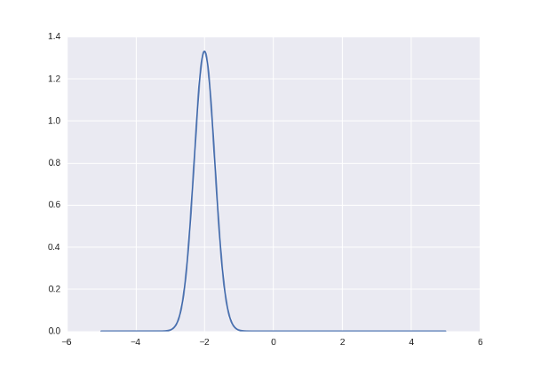
Accordingly, the numbers that correspond to this distribution (live in a neighborhood of -2) will be considered “correct” and “original”, while the others will not.

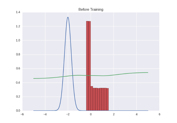
Take Theano and Lasagne, and define our models - simple neural networks with two layers of ten neurons each. At the same time, because of the mechanism of the Theano operation (it builds a symbolic graph of calculations and allows you to specify one specific variable as the discriminator input, we need two originals and fakes) to make two copies of the discriminator: one will pass through the “correct” numbers, and the second is generator fakes.



Let's draw a picture of how the discriminator behaves - that is, for each number that is on the line (we limit ourselves to the range from -5 to 5), we note the discriminator's confidence that this number is correct. We will get the green curve on the graph below - as you can see, since the discriminator is not trained in us, it gives out a full house-house heresy. And at the same time we ask the generator to spit out a certain number of numbers and draw their distribution using a red histogram:



And a little more Theano-code to make the price function and start learning:



We use here the learning rate decay and not a very big momentum. In addition, the discriminator trains several steps one generator step (20 in this case) - a somewhat muddy point about which there is in the article, but it is not very clear why. My guess is that this allows the generator to not react to random throwing of the discriminator (i.e., the counterfeiter first waits until the banker approves the strategy of behavior for himself, and then tries to deceive it).

The learning process looks like this:



What happens in this gif? The green line tries to push the red histogram into the blue contour. When the discriminator's limit in a certain place falls below 0.5, this means that for the corresponding places the numerical direct discriminator suspects more fakes than the originals, and will rather produce negative conclusions (thus, it almost pushes outliers of red numbers). to the right of the distribution center after the first few seconds gifs)

Where the histogram coincides with the contour, the discriminator curve stays at 0.5 — this means that the discriminator can no longer distinguish counterfeits from the originals and does the best that it can in such a situation — it just randomly spits guesses with the same probability.

Outside the area of ​​interest to us, the discriminator behaves not very adequately - for example, it positively classifies all numbers greater than -1 with a probability of ~ 1, but this is not terrible, because in this game we support the counterfeiter and it is his success that interests us.

This couple is curious to watch, playing with different parameters. For example, if you put momentum too large, both participants in the game will begin to respond too sharply to the learning signals and correct their behavior so much that they make it even worse. Something like this:



The entire code can be viewed here .

An example is more interesting

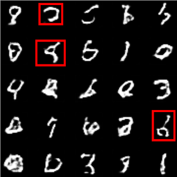
Well, it was not so bad, but we are capable of more, as the title picture hints. Let's try the newfound skills of the counterfeiter on the good old handwritten numbers.

Here, the generator will have to use a little trick, which is described in the article codenamed DCGAN (they are also used by Lars and Soren in the title post). It consists in the fact that we do such a kind of convolutional network, vice versa (a sweep network?), Where we replace subsampling layers that reduce the image N times with upsampling layers that increase it, and do convolutional layers in full mode - when the filter jumps out of the picture and at the output gives more result than the original picture. If this is dull and unclear for you, this page will clarify everything in five minutes, but for now you can remember a simple rule - in the case of the usual convolution by filter the result will have a side , and full convolution - . This will allow us to start with a small square of noise and "expand" it into a full-fledged image.



The generator code for the MNIST numbers looks something like a spoiler. The discriminator is some simplest convolutional network. To be honest, I one-to-one tore it from the Las Casmeme's readme, and I won't even bring it here.



The result is something like this.



Not exactly perfect, but something definitely similar. It's funny to watch how the generator first learns to draw with similar strokes, and then struggles a decent time in order to make a regular shape of them. For example, here the selected characters do not look like numbers, but they clearly represent some kind of characters, that is, the generator went the right way:



Going further, we take the LFW Crop face database, first we reduce the faces to the size of MNIST (28x28 pixels) and try to repeat the experiment, only in color. And immediately notice several patterns:

1) Persons train worse. The number of neurons and layers that I brought here for MNIST is taken slightly with a margin - it can be halved, and it will turn out well. Persons at the same time turn into an incomprehensible random mess.
2) Colored faces train even worse - which is understandable, of course, the information becomes three times more.
3) Sometimes it is necessary to correct the mutual behavior of the generator and the discriminator: there are situations when one drives the other into a dead end, and the game stops. This usually happens in a situation where, say, the discriminator is more powerful in a representative sense — it can understand such fine details that the generator is still (or not at all) able to distinguish. Again, the title post describes several heuristics (slow down the discriminator when it gets too good grades, etc.), but everything worked quite well without me - I had enough to correct the settings and the number of neurons at the beginning of the training.

And the result:



Not bad, not bad, but I still want something of the same quality as on the KDPV!

Full-size example and walk in recipe space

I loaded the regretful GT 650M with a full-sized (64x64) LFW Crop and left it overnight. Approximately 30 eras (per 10,000 persons) passed by morning, and the end result looked like this:



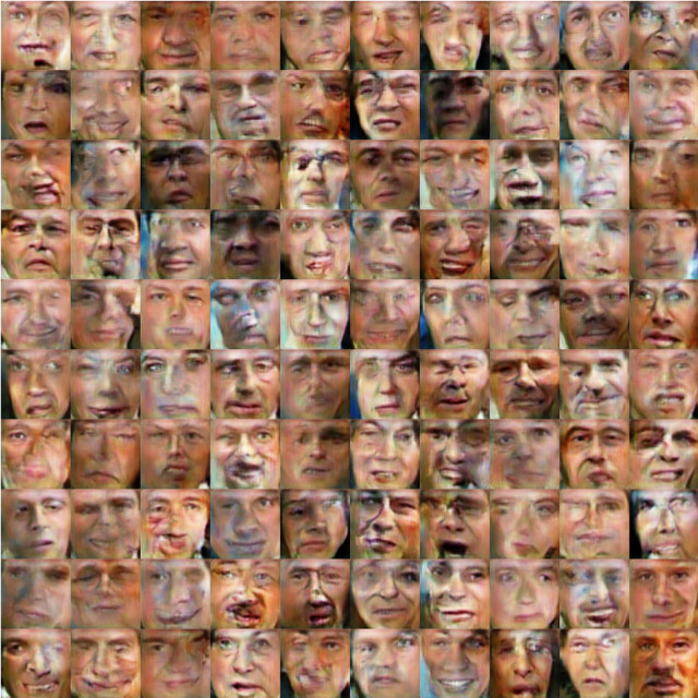
What a beauty. If anyone needs character portraits for a zombie apocalypse, let me know! I have a lot of them.
The quality was not very good, but something similar to the situation with MNIST happened - our generator learned to cope with visual noises and vagueness, to draw eyes, noses and mouths properly, and now he has a problem called “how to combine them correctly”.

Let's now think again what we have drawn. All these faces are spat out by the same network, and a neural network is a deterministic thing through and through, just a sequence of multiplications and additions (and nonlinearities, okay). I did not add any randomization, dropout, etc. to the generator. So how do people get different? Obviously, the only source of randomization that the network can use is the same input noise that we used to call the “meaningless” parameter. Now it turns out that it turns out to be quite important - in this noise all the parameters of the output face are encoded, and all that the rest of the network does is simply read the input “recipe” and apply paint according to it.

And the recipes are not discrete (I did not have time to say about this, but a simple uniform distribution of numbers from 0 to 1 was taken as noise). True, we still do not know what number in the recipe is what exactly encodes, hmm - and even "does something meaningful encode any single number?" Well, why do we need all this then?

First, knowing now that the input noise is a recipe, we can control it. Uniform noise, to put it bluntly, was not a very good idea - now every bit of noise can encode anything with the same probability. We can apply to the input, say, normal noise (distributed over Gauss) - then noise values ​​close to the center will occur frequently and encode something common (such as skin color), and rare outliers something special and rare ( for example, glasses on the face). People who wrote the DCGAN article found a few semantic pieces of the recipe, and used them to put glasses on people or make them frown at will.

Secondly ... have you seen the meme on “image enhancing” from the CSI series? A thing that all people who are familiar with computers have long laughed at: the powerful FBI algorithm magically increases the resolution of the picture. So, we may still have to take our words back, because why not make our generator's life a little easier, and instead of giving noise to the input, give, say, a smaller version of our original? Then, instead of drawing faces from the head, the generator will just have to “draw them” - and this task clearly looks simpler than the first one.

I, unfortunately, did not reach this point, but here there is an excellent post demonstrating how this is done with impressive illustrations.

Well and thirdly, you can have some fun. Since we know that recipes are not discrete, there are transition states between any two recipes. We take two noise vectors, interpolate them and feed the generator. Repeat, until you get bored, or until the people in the room seriously start to worry, why are you looking at agonizing zombies so closely.

Conclusion

1) Adversarial networks are fun.
2) If you decide to try to train them yourself - it is easier to peek at the ready-made recipes than to play with the parameters.
3) Joshua Bengio named DCGAN and LAPGAN (which is image enhancing) among the most impressive pieces in machine learning in 2015 and it was after this that I read about them, of course
4) Another blog was recently a good post on the topic of “deep learning is easy, try something harder” - just for people like me who are hooked on a popular topic and don’t really know where to go next. Adversarial networks is a good option (and also mentioned in the post as one of the new promising areas), because there are a lot of interesting things, and control over the recipes is only one of the most promising things.
5) How to translate "adversarial networks" into Russian? "Warring networks"? "Rival networks"?