On Habré and beyond, they often discuss relational algebra and SQL, but far less often focus on the connections between these formalisms. In this article, we will go to the very roots of query theory: relational calculus, relational algebra, and the SQL language. We will analyze them with simple examples, and also see that it can be useful to switch between formalisms for analyzing and writing queries.

Why might it be needed today? Not only data analysts and database administrators have to work with data, in fact very few people don’t have to extract something from (semi-) structured data or transform existing ones. In order to have a good idea why query languages ​​are arranged in a certain way and consciously use them, you need to deal with the underlying core. We will talk about this today.
')
Most of the articles are examples interspersed with theory. At the end of the sections are links to additional materials, and for those interested, and a small selection of literature and courses at the end.

Content

• Relational algebra
• SQL
• Relational calculus
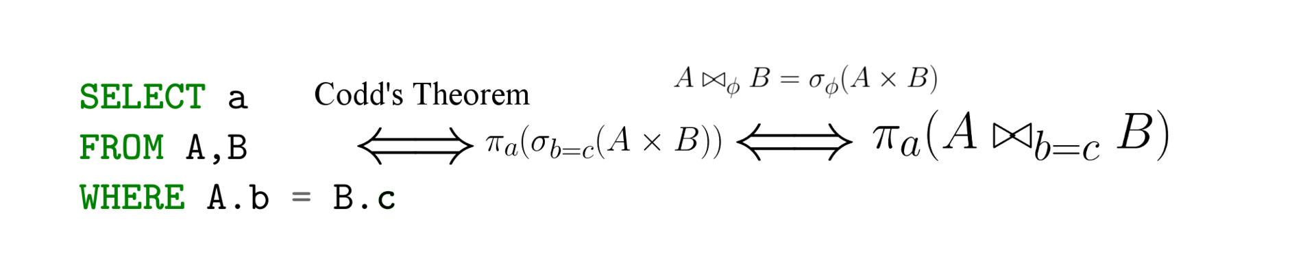
• Equality of Formalisms (Codd's Theorem)
• Conjunctive Queries (CQ)
• Computational complexity
• Query properties and analysis
• An example of using RA to optimize queries
• Literature, materials and slides

Relational algebra

Main operators

- the relation A itself (the relation here is synonymous with a table and a predicate) is an expression of relational algebra, moreover, since it is an algebra, any expression of a relational algebra returns a relation (the closure property of operators)

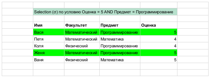
Selection (selection; restriction)

- selection (selection; restriction), A - relation (predicate, table), - Boolean formula by which the selection of lines (tuples, records, etc)

Selection is essentially a horizontal line filter, i.e., you can imagine that we go along each line and leave only those that satisfy the condition . A simple example for clarity:

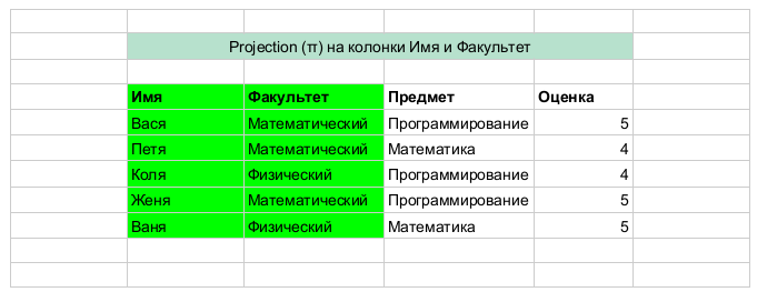
Projection

- projection on the attributes A, B, .... Returns a table in which only columns (attributes) A, B, ... remain. A simple example is below. In essence, it is a filter by attributes i. it is in a sense a vertical filter.

Rename

- renames the column a to b in relation to A (attribute, predicate argument, etc); two teas to the gentleman who will show that algebra is strictly more expressible with the renaming operator (we need to give an example of a query that we cannot express without this operator, but we will express it with )

Cartesian product

- Cartesian product of two relations, a large ratio of all possible combinations of strings in A and B.

Set operations

Relational algebra is an extension of the classical set of operators over sets (a relation is a set of ordered tuples; note that this is not at all equal to the ordered set of tuples). Suppose we have a table StudentMark (Name, Mark, Subject, Date) - then the tuple (Vasya, 5, Informatics, 10/05/2010) is ordered - first the string Name on the first (ok, or zero) position, an integer on the second, line on the third and date on the fourth. At the same time, the ordered tuples themselves (Name, Mark, Subject, Date) are not ordered “within” the relationship.

Union

- union of all strings in A and B, restriction - identical attributes

Intersection

- the intersection of lines, the same restriction

Set difference

- B minus A, all strings that are present in B, but not in A, the same restriction

(B \ A; A - on the left, B - on the right)

Auxiliary operators

- join (connection); join joins two records of tables A and B, provided that the condition φ is met for these two records.

Tasks for warming up

We will work with the following scheme.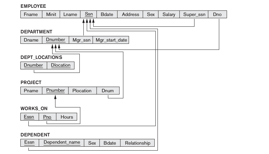

(The diagram is taken from the book: Elmasri, Navathe - Fundamentals of Database systems; for everyone: I highly recommend NOT the book; see the selection at the end)

Next, we consider several simple problems on relational algebra.

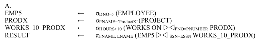
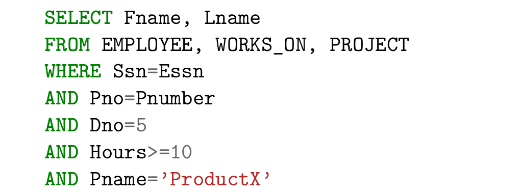
Task one. Print the names of all 5th Department employees who work more than 10 hours a week on Project X.

(Intermediate results can be “preserved” in new relationships, but this is not necessary.)

Task two. Print the names of all employees directly supervised by Franklin Wong (and find a small mistake in the decision below)

The third task will require the use of a new operator - “aggregation”. Consider it by example:

For each project, print the name and total number of hours per week that all employees spend on this project.

Note that the query has the form a F b (A), where a, b are columns, A is a relation, and a is an aggregation function (for example, SUM, MIN, MAX, COUNT, etc). It reads as follows: for each value in column a, count b. That is, one value in column a can correspond to several lines, put the values ​​of column b from this set of lines in the function and create a new attribute fun_b with the appropriate value.

This query cannot be expressed in a “classical” relational algebra (without the aggregation operator F). That is, you cannot write a single query that, for any database that satisfies the schema, gives the correct answer.

From where exactly the given result follows, we will analyze later; now we can only note that requests with aggregation belong to a higher class of computational complexity.

We will consider and analyze more interesting examples of problems later in the article. There's also a small selection of problems on relational algebra with solutions available here.

SQL

In this part we will talk about SQL (Structured Query Language) and show how SQL corresponds to relational algebra with simple examples.

Consider the very first task again:

Task one. Print the names of all 5th Department employees who work more than 10 hours a week on Project X.

The classic solution is as follows:

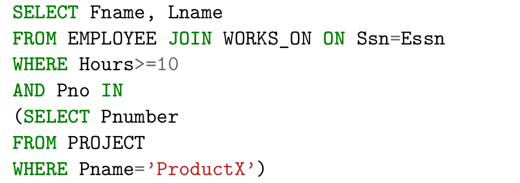
Alternatively, you can write this:

Or quite alternatively:

(further solutions are not removed under spoilers)

Draw an analogy between SQL and relational algebra

In the second solution, we see a distinct analogy with relational algebra:

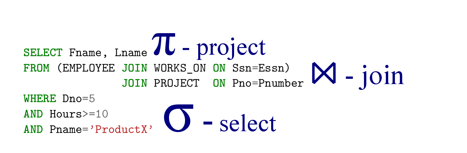
Now use equality for join and see the analogy between SQL and relational algebra in the first solution

No matter how ironic it is, but SELECT in SQL is the project (π; projection) in relational algebra.

Now consider the problem with aggregation and compare it with the solution on relational algebra:

We will look at more interesting problems later in the article (also a small selection here ), and now we will consider another query formalism.

Relational calculus

Attentive reader now could exclaim: why goat bayan? What we lack here is two formalisms for writing queries, what is the third one for?

Relational calculus is an adaptation of first order logic (FOL: first order logic) for writing queries. FOL is one of the most well-studied formalisms of mathematics and makes it possible to use the already created theoretical apparatus and classical results for analyzing and writing queries.

Many results in complexity, (not) expressibility and formation of queries came to the database from logic, precisely because of relational calculus, therefore it is worth getting acquainted with this formalism.

To parse and talk about relational calculus, we need first-order logic, which can be refreshed here .

Let φ (X) be a first-order formula, and X are free variables, that is, they are not quantified (∀ is a universal quantifier, is an existence quantifier), then the query in relational calculus defines a set:

{X | φ (X)}

Consider simple examples on which we analyze the formalism:

Let R be a relation with three attributes a, b, c; then rewrite the following query of relational algebra:

in relational terms like:

{ra, rb, rc | R® and ra = rc}

Translating into simple language r is a tuple in R (that is, a string with attributes whose values ​​can be obtained through a point by name, ie, ra is an attribute of a tuple r (strings) with respect to R (table)). As we see, there are no quantifiers here, since r is at the output of the query and should be a free tuple.

Consider another simple example: R (a, b, c) ∗ S (c, d, e), where * is a natural join, i.e. join by name - as the join condition, take attributes with the same name.

{rA, rB, rC, sD, sE | R® and S (s) and rC = sC}

If sD and Se were not among the output parameters, the request would have the following form:

{rA, rB, rC | R® and ∃s: S (s) and rC = sC}

We would be obliged to put a quantifier of existence, since S is contained only in the "body" of the request.

When making such queries, you should always be careful with the quantifier of universality if we write the following expression (for illustration purposes only):

{rA | R® and ∀s: S (s) and rC = sC and sE = “banana”}

That, this query will always return an empty set, since in order for the query conditions to be fulfilled it is necessary that every tuple in the world of length three belongs to S and has the value of the last attribute “banana”.

Usually, together with the universal quantifier, the implication “=>” is used, we can rewrite the query as follows:

{rA | R® and ∀s: (S (s) and rC = sC) => sE = "banana"}

If s belongs to S and the value of C is the same as C in R, then the last attribute should have the value banana.

Here you can find a short selection of problems on relational calculus with solutions.

Equality of Formalisms (Codd's Theorem)

In simple terms, Codd's theorem sounds like this: all three SQL formalisms, relational algebra, and relational calculus are equal. Here is a lot of theory for those interested.

That is, any query expressed in one language can be reformulated in another. This result is primarily convenient in that it allows the use of the most convenient formalism for analyzing a query, and secondly it connects declarative SQL languages ​​and relational calculus with imperative relational algebra. That is, by translating a query from SQL to relational algebra, we already get a way to execute the query (and optimize it).

Conjunctive Queries (CQ)

Requests that consist of a select (σ) -project (π) -join (⋈) segment of relational algebra are called conjunctive queries (ok, I omitted renaming, we consider it implicitly present).

If you have read this line, try to solve the following problem using only these three operators (and of course the relationship):

Task. Print the names of all the workers who work on each project.

Consider which segment of SQL and relational calculus this class of relational algebra belongs to.

Computational complexity

There are several different ways to measure the computational complexity of the query, between them are often confused therefore write out the definitions and their names:

Let Q is a query, D is a database, and you need to calculate Q (D)

• If Q is fixed, then the complexity of the calculation of f (D) is called data complexity (data complexity)
• If D is fixed, then the complexity of the calculation of f (Q) is called the complexity of the query (query complexity)
• If nothing is fixed, then the complexity f (Q, D) is called the combined complexity (combined complexity)

Important facts: SQL complexity by data (and all the others) belongs to the class AC0 - this is a very good complexity class, i.e., queries can be calculated very effectively.

From a theoretical point of view, you can look at this picture here:

AC0 lies within NL (more precisely, even within one of the NC layers within NL).

Consider the following interesting question related to computational complexity: let f be a function of the satisfiability of a formula, that is, for each query, it says whether a database exists such that Q (D) is true. From the Codd theorem, we know that relational algebra and SQL are equivalent to relational calculus. So, the calculation of f is equivalent to the stopping problem (the SAT for the first order logic is not computable). From here: there are no algorithms that, for an arbitrary SQL query, could determine its consistency.

For those interested, I also recommend: Trakhtenbrot theorem

Difficulty Conjunctive Queries

CQs are one of the most studied classes of queries as they make up the bulk of database queries (I saw a figure of 90% on one presentation, but I can’t find the source now). Therefore, we consider in more detail their complexity and prove that in reality their combined complexity is equal to NP, i.e. The task is NP complete. (You can read about full NP here and here .)

To do this, we write an arbitrary CQ query in relational calculus in the form:

{X | [∃X0:] p0 (X0) and [∃X1:] p1 (X1) and [∃X1:] p (X2) ...}

Where [.] Is an optional quantifier. Why is such a representation always permissible? Because the project here can always be expressed in X i. , join is expressed in terms of equality of variables in , and select through conditions on in the request body.

To show that the task belongs to the class NP-complete, you need to do two things.

• Show that task inside NP class
• Show that NP is a complete task comes down to this

The first condition is trivial: since the values ​​of relations are finite (that is, the set of all possible values), we can “guess” the function nondeterministic such that makes each relationship true under the quantifiers of existence.

We show that the graph coloring problem is reduced to the problem of the feasibility of a CQ query.

Let D consist of one relation edge = {(red, green), (green, red), (blue, red), (green, blue) ...} - all possible correct colorings of the graph, such that no two vertices have the same color .

Let the original graph be given as a set of edges

Then, we write the following query

{() | ∃X0 ... ∃XN: edge (V1, V2) and ... edge (V_i, V_j) ...}

That is, each arc in the source graph in the query will correspond to an edge relation with the corresponding arguments. If the request returned an empty tuple, it means that there is such a function. that displays , and no two vertices will have the same color (follows from the definition of D). C.T.D.

Question with an asterisk: from the select-project-join segment we throw out the project, how will the computational complexity change?

Transitive closure

Determining the complexity of the data and on request also shed light on one known result - in classical SQL (without with) the transitive closure is inexpressible with a fixed query ie. you cannot write a single query such that for any database it would calculate the predicate closure. That is, if we have a graph saved as an edge relationship, then we cannot write one fixed query that would calculate the reachability relation for an arbitrary graph. Although intuitively it seems that such a query should clearly lie in the class CQ.

This can be seen either from computational complexity “by data”, or it is much more constructive and interesting that follows from the compactness theorem and Codd's theorem (SQL = First Order Logic).

The proof is non-trivial and can be skipped without losing the understanding of further material.


If the query is not fixed, then the problem becomes trivially solvable. Let me have only k edges in the database, it means the largest path is no more than k, it means that you can write the query in an explicit form, as a union of paths of length 1, 2, ... k and thus get a query that computes reachability in the graph.

Query properties and analysis

Now back to the task proposed earlier:

Print the names of all the workers who work on each project.

Why this problem has no solution in the CQ class we can understand by defining the key properties of the query itself and the CQ class.

The definition, the query Q is called monotonous, if and only if, for any two databases right that . That is, an increase in the database can only increase the number of tuples in the output or remain the same.

Observation: CQ is a class of monotonically increasing queries. Imagine an arbitrary CQ request Q - it consists of select-project-join. Let us show that each of them is a monotone operator:

Suppose we have added another entry in D

• select - filters records vertically, if a new record satisfies the query, then the set of answers increases, if not, it remains the same.

  
  

• project - does not affect the additional tuple

  
  

• join - if the corresponding record is also in the second set, then the response set will expand, otherwise it will remain the same.

  
  

Superposition of monotone operators monotone => CQ is a class of monotonous queries.

Question: Is the original task monotonous? Not really. Suppose we have only one employee Petya, who is working on two projects A and B, and we have 2 projects A and B in total, which means Petya must be in issuing a request. Suppose we added the third project C => now Petit is not in the answer and the response set is empty, which means the request is not monotone.

The following question logically follows from this: what do you need to add to the select-project-join so that the problem is solved? This is something that should be non-monotonic!

As of course, the reader guessed - the difference of sets. His asymmetry seemed to tell us and set it apart from the very beginning.

However, before writing a solution, we make one more observation: if there are no counter-examples to the statement, this statement is always true. Formally:

- there is no x such that p (x) is incorrect.

In the task, we see an explicit “for all” quantifier and we can emulate it using double negative, that is, we rephrase the query as follows: output the names of all employees for whom there is no project on which they would not work

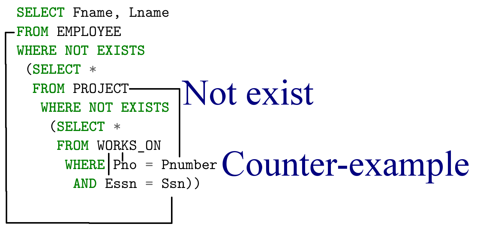
This same query looks incredibly simple if we had (and it is in relational calculus):

{e.fname, e.lname | EMP (e) and PRJ (p) WORKS_ON (w) and w.Pno = p.Pnumber and e.Ssn = w.Essn}

An example of using RA to optimize queries

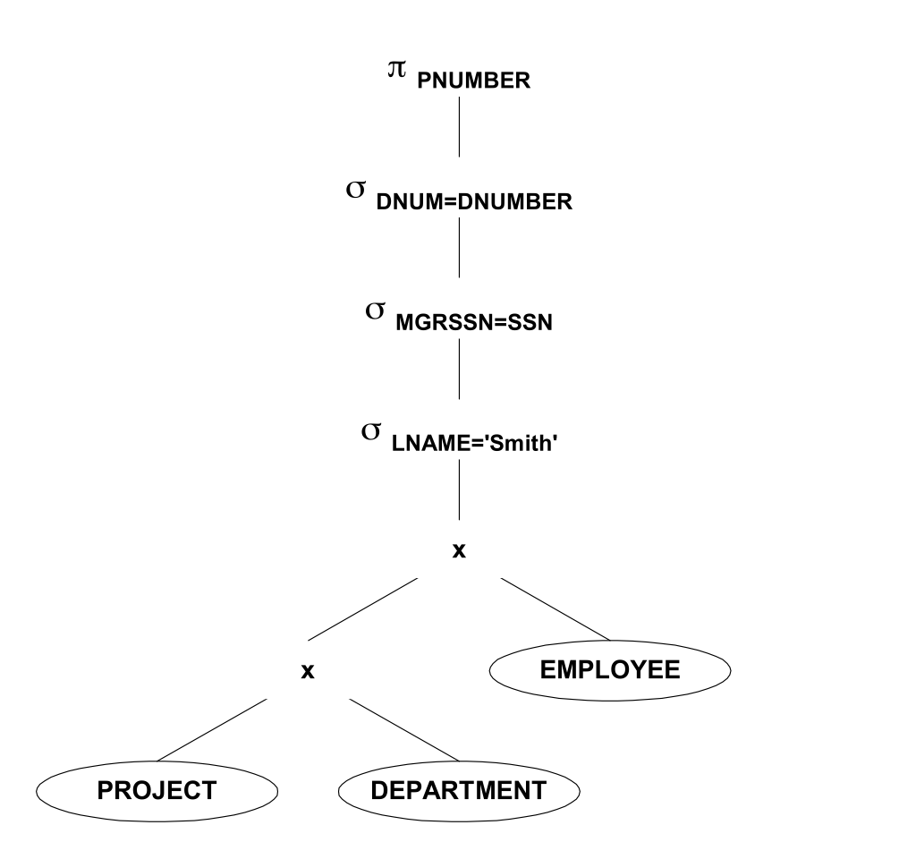
Transforming SQL into relational algebra also optimizes query execution. Consider a simple example:

Task
Print all the numbers of projects in which the employee with the surname Schmidt worked as the manager of the department managing this project.

A simple solution is as follows: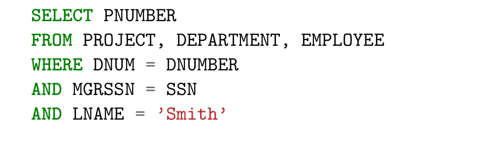

Which can be rewritten into relational algebra as follows:

The first optimization is to use select as early as possible, then the Cartesian product will receive smaller relations as input:

Select c equality constant strong constraint, so it must be calculated and connected as soon as possible: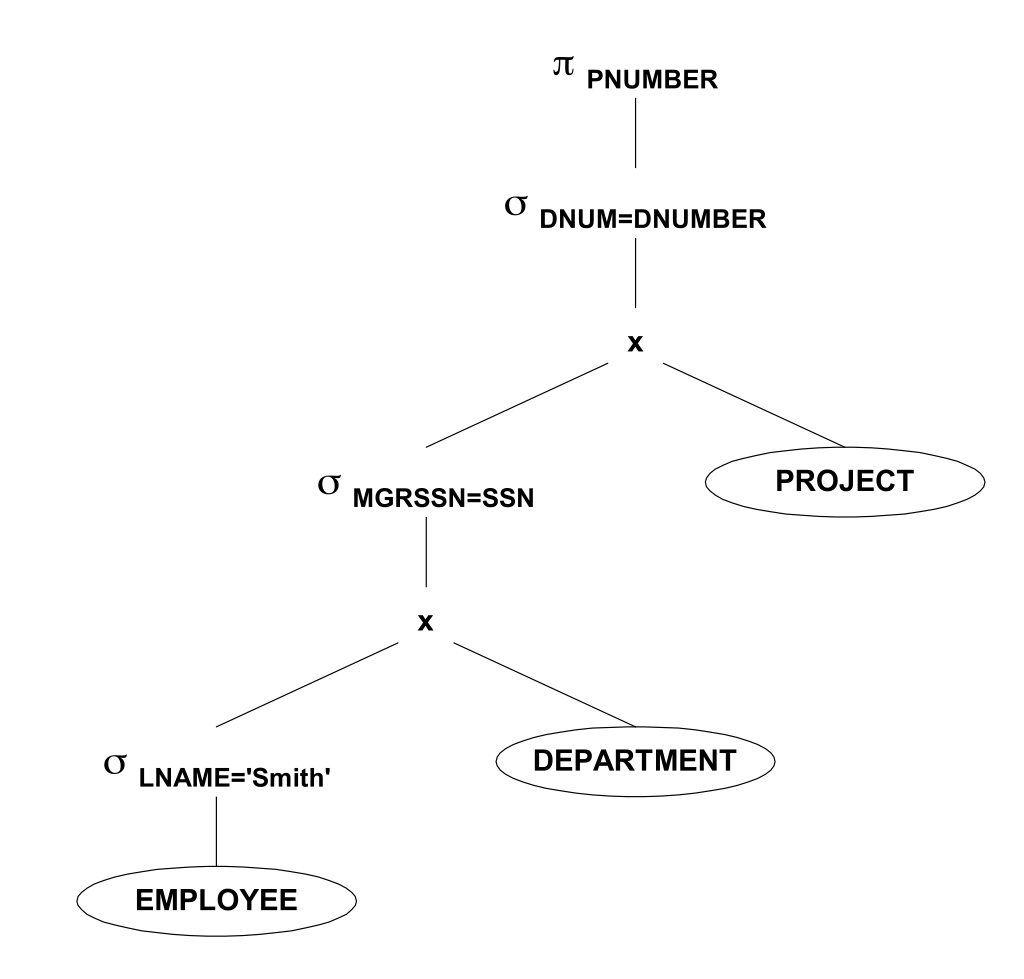

We collapse the Cartesian product and select into a join (which is implemented effectively with indices and specialized data structures)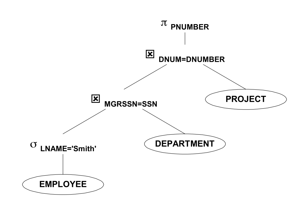

Drop the project as low as possible so that only the necessary information is passed up the tree.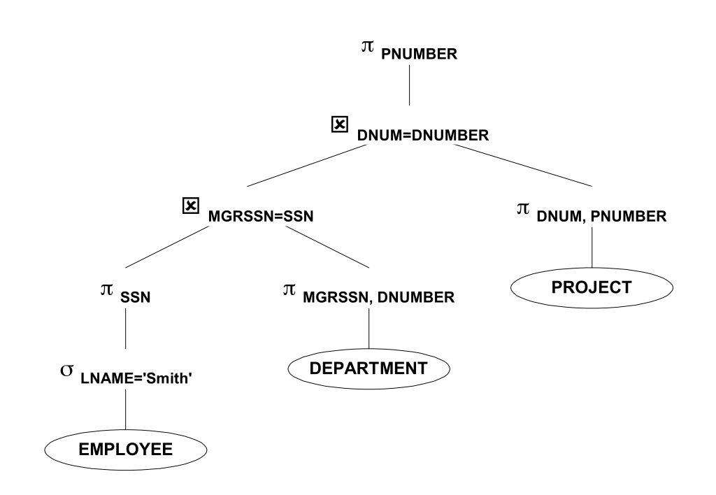

Literature, materials and slides

Stanford online course - Jennifer Widom - excellent course, I recommend

Alice's book - Serge Abiteboul - classics of the genre

Martin Graber - SQL - fairly simple and detailed explanations of the work of algorithms and SQL syntax

Habra articles about P-NP - introductory material part one and two

My slides on the topic (extremely useful because of the examples of problem solutions in different formalisms - in some places a mixture of Dutch and English)

Good slides on the theory (non-trivial theoretical material)