Monte Carlo method and its accuracy
Metd Monte Carlo means numerical solution.
math problems using random variable simulation. An idea of the history of the method and the simplest examples of its use can be found in Wikipedia .
In the method itself there is nothing difficult. It is this simplicity that explains the popularity of this method.
The method has two main features. The first is the simple structure of the computational algorithm. The second is a calculation error, usually proportional
 where
where  - some constant, and
  - the number of tests. It is clear that to achieve high accuracy on this path is impossible. Therefore, it is usually said that the Monte Carlo method is especially effective in solving those problems in which the result is needed with a little accuracy.
')
However, the same problem can be solved by different versions of the Monte Carlo method, which correspond to different values . In many problems, it is possible to significantly increase the accuracy by choosing a method of calculation, which corresponds to a significantly lower value. .
Suppose we need to calculate some unknown quantity m. Let's try to invent such a random variable. so that
  . Let at the same time
  .
.
Will consider independent random variables  (implementations) whose distributions coincide with the distribution . If a is large enough, then according to the central limit theorem the distribution of the sum
  will be approximately normal with parameters
  ,
,  .
.
On the basis of the Central Limit Theorem (or, if you wish, the Muavre-Laplace limit theorem), it is not difficult to obtain the relation:
%3DP%5Cleft(%20%5Cleft%7C%20%5Cfrac%7B1%7D%7BN%7D%5Csum%5Climits_%7Bi%7D%7B%7B%7B%5Cxi%20%7D_%7Bi%7D%7D%7D-m%20%5Cright%7C%5Cle%20k%5Cfrac%7Bb%7D%7B%5Csqrt%7BN%7D%7D%20%5Cright)%5Cto%202%5CPhi%20(k)-1%2C)
Where) - distribution function of the standard normal distribution.
- distribution function of the standard normal distribution.
This is an extremely important relation for the Monte Carlo method. It gives the calculation method , and an error estimate.
In fact, we find random values  . From this ratio, it is clear that the arithmetic average of these values will be approximately equal to . With probability close to
 -1)) the error of such an approximation does not exceed the magnitude
the error of such an approximation does not exceed the magnitude  . Obviously, this error tends to zero with increasing .
Depending on the goals, the last relation is used in different ways:
As can be seen from the above ratios, the accuracy of the calculations depends on the parameter and values  - standard deviation of a random variable .
At this point, I would like to indicate the importance of the second parameter. . This is best shown by example. Consider the calculation of a definite integral.
The calculation of a definite integral is equivalent to the calculation of areas, which gives an intuitively clear algorithm for calculating the integral (see the Wikipedia article). I will consider a more effective method (a special case of the formula for which, however, is also in the article from Wikipedia). However, not everyone knows that instead of a uniformly distributed random variable, this method can use almost any random variable specified on the same interval.
So, it is required to calculate a certain integral:
dx%7D)
Choose an arbitrary random variable with distribution density ) determined on the interval
determined on the interval ) . And consider the random variable
. And consider the random variable %2F%7B%7Bp%7D_%7B%5Cxi%20%7D%7D(%5Cxi%20)) .
.
The expected value of the last random variable is:
![M \ zeta = \ int \ limits_ {a} ^ {b} {[g (x) / {{p} _ {\ xi}} (x)] {{p} _ {\ xi}} (x) dx = I}](http://tex.s2cms.ru/svg/M%5Czeta%20%3D%5Cint%5Climits_%7Ba%7D%5E%7Bb%7D%7B%5Bg(x)%2F%7B%7Bp%7D_%7B%5Cxi%20%7D%7D(x)%5D%7B%7Bp%7D_%7B%5Cxi%20%7D%7D(x)dx%3DI%7D)
Thus, we get:
%5Capprox%200.9973.)
The last ratio means that if you choose values then at a sufficiently large :
%7D%7B%7B%7Bp%7D_%7B%5Cxi%20%7D%7D(%7B%7B%5Cxi%20%7D_%7Bi%7D%7D)%7D%5Capprox%20I%7D) .
.
Thus, to calculate the integral, you can use almost any random variable. . But dispersion , and with it the accuracy estimate, depends on which random variable take for calculations.
It can be shown that will have a minimum value when proportional to | g (x) |. Choose such a value In the general case, it is very difficult (complexity is equivalent to the complexity of the problem being solved), but it is worth being guided by this consideration, i.e. choose a probability distribution in the form similar to the module of the integrable function.
The theory, of course, is a good thing, but let's look at a numerical example: ;
;  ;
; %3Dcos(x)) .
.
We calculate the value of the integral using two different random variables.
In the first case, we will use a uniformly distributed random variable on [a, b], i.e.%3D2%2F%5Cpi%20) .
.
In the second case, we take a random variable with a linear density on [a, b], i.e.%3D%5Cfrac%7B4%7D%7B%5Cpi%20%7D(1-2x%2F%5Cpi%20)) .
.
Here is a graph of the specified functions.
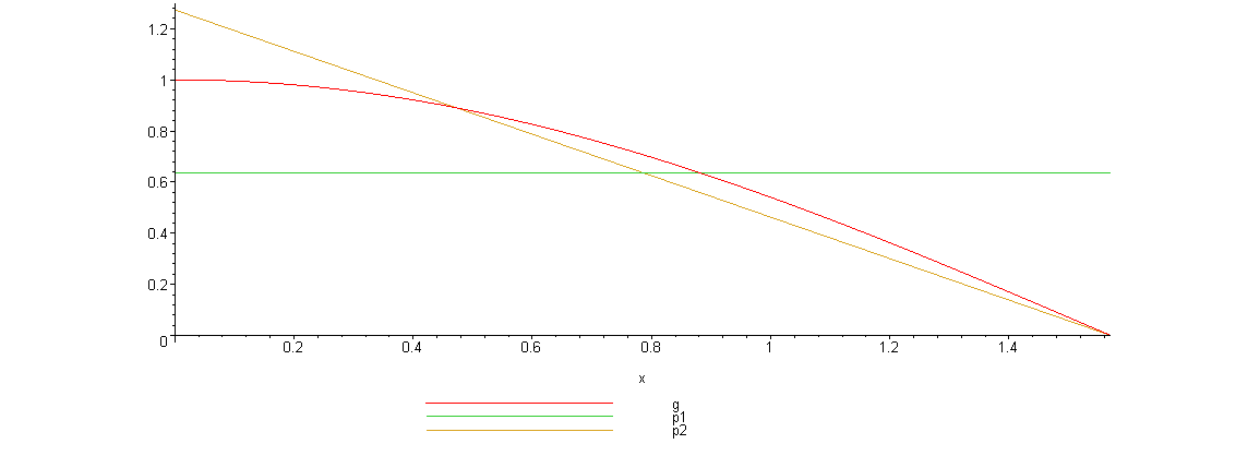
It is easy to see that the linear density better matches the function.) .
.
The exact value of the integral is easy to calculate analytically, it is equal to 1.
The results of one simulation with :
:
For a uniformly distributed random variable: .
.
For a random variable with a linear distribution density: .
.
In the first case, the relative error is more than 21%, and in the second 2.35%. Accuracy in the first case it is equal 0.459, and in the second - 0.123.
I think this model example shows the importance of choosing a random variable in the Monte Carlo method. By choosing the correct random value, you can get a higher accuracy of calculations, with fewer iterations.
Of course, one-dimensional integrals are not calculated this way, there are more accurate quadrature formulas for this. But the situation changes during the transition to multidimensional integrals, since quadrature formulas become cumbersome and complex, and the Monte Carlo method is applied only with minor modifications.
It is not difficult to see that the accuracy of the calculations depends on the number random variables included in the amount. Moreover, to increase the accuracy of calculations 10 times you need to increase 100 times.
When solving some problems, it is necessary to take a very large number to obtain an acceptable accuracy of the estimate. . And given that the method often works very quickly, then implementing the latter with modern computing capabilities is not at all difficult. And the temptation is to simply increase the number .
If a physical phenomenon is used as a source of randomness (a physical sensor of random numbers), then everything works fine.
Often, pseudo-random number sensors are used for Monte-Carlo calculations. The main feature of such generators is the presence of a certain period.
The Monte Carlo method can be used with values not exceeding (preferably a lot smaller) the period of your pseudo-random number generator. The latter fact follows from the condition of independence of random variables used in modeling.
For large calculations, you need to make sure that the properties of the random number generator allow you to do these calculations. In standard random number generators (in most programming languages), the period most often does not exceed 2 in the degree of bitness of the operating system, or even less. When using such generators, one must be extremely careful. It is better to study the recommendations of D. Knut, and build your own generator, which has a known and sufficiently long period in advance.
Popular lectures on mathematics 1968. Issue 46. Sobol I.M. Monte Carlo method. M .: Science, 1968. - 64 p.
math problems using random variable simulation. An idea of the history of the method and the simplest examples of its use can be found in Wikipedia .
In the method itself there is nothing difficult. It is this simplicity that explains the popularity of this method.
The method has two main features. The first is the simple structure of the computational algorithm. The second is a calculation error, usually proportional
')
However, the same problem can be solved by different versions of the Monte Carlo method, which correspond to different values
General scheme of the method
Suppose we need to calculate some unknown quantity m. Let's try to invent such a random variable.
Will consider
On the basis of the Central Limit Theorem (or, if you wish, the Muavre-Laplace limit theorem), it is not difficult to obtain the relation:
Where
This is an extremely important relation for the Monte Carlo method. It gives the calculation method
In fact, we find
Depending on the goals, the last relation is used in different ways:
- If we take k = 3, we get the so-called “rule
":
- If a specific level of computation reliability is required
,
Calculation accuracy
As can be seen from the above ratios, the accuracy of the calculations depends on the parameter
At this point, I would like to indicate the importance of the second parameter.
The calculation of a definite integral is equivalent to the calculation of areas, which gives an intuitively clear algorithm for calculating the integral (see the Wikipedia article). I will consider a more effective method (a special case of the formula for which, however, is also in the article from Wikipedia). However, not everyone knows that instead of a uniformly distributed random variable, this method can use almost any random variable specified on the same interval.
So, it is required to calculate a certain integral:
Choose an arbitrary random variable
The expected value of the last random variable is:
Thus, we get:
The last ratio means that if you choose
Thus, to calculate the integral, you can use almost any random variable.
It can be shown that
Numerical example
The theory, of course, is a good thing, but let's look at a numerical example:
We calculate the value of the integral using two different random variables.
In the first case, we will use a uniformly distributed random variable on [a, b], i.e.
In the second case, we take a random variable with a linear density on [a, b], i.e.
Here is a graph of the specified functions.
It is easy to see that the linear density better matches the function.
The program code of the model example in the mathematical package Maple
The file with this program can be found here.
restart; with(Statistics): with(plots): # g:=x->cos(x): a:=0: b:=Pi/2: N:=10000: # p1:=x->piecewise(x>=a and x<b,1/(ba)): p2:=x->piecewise(x>=a and x<b,4/Pi-8*x/Pi^2): # plot([g(x),p1(x),p2(x)],x=a..b, legend=[g,p1,p2]); # I_ab:=int(g(x),x=0..b); # - # INT:=proc(g,p,N) local xi; xi:=Sample(RandomVariable(Distribution(PDF = p)),N); evalf(add(g(xi[i])/p(xi[i]),i=1..N)/N); end proc: # I_p1:=INT(g,p1,N);#c I_p2:=INT(g,p2,N);#c # Delta1:=abs(I_p1-I_ab);#c Delta2:=abs(I_p2-I_ab);#c # delta1:=Delta1/I_ab*100;#c delta2:=Delta2/I_ab*100;#c # Dzeta1:=evalf(int(g(x)^2/p1(x),x=a..b)-1); Dzeta2:=evalf(int(g(x)^2/p2(x),x=a..b)-1); # 3*sqrt(Dzeta1)/sqrt(N); # 3*sqrt(Dzeta2)/sqrt(N); The file with this program can be found here.
The exact value of the integral is easy to calculate analytically, it is equal to 1.
The results of one simulation with
For a uniformly distributed random variable:
For a random variable with a linear distribution density:
In the first case, the relative error is more than 21%, and in the second 2.35%. Accuracy
I think this model example shows the importance of choosing a random variable in the Monte Carlo method. By choosing the correct random value, you can get a higher accuracy of calculations, with fewer iterations.
Of course, one-dimensional integrals are not calculated this way, there are more accurate quadrature formulas for this. But the situation changes during the transition to multidimensional integrals, since quadrature formulas become cumbersome and complex, and the Monte Carlo method is applied only with minor modifications.
Number of iterations and random number generators
It is not difficult to see that the accuracy of the calculations depends on the number
When solving some problems, it is necessary to take a very large number to obtain an acceptable accuracy of the estimate.
If a physical phenomenon is used as a source of randomness (a physical sensor of random numbers), then everything works fine.
Often, pseudo-random number sensors are used for Monte-Carlo calculations. The main feature of such generators is the presence of a certain period.
The Monte Carlo method can be used with values
For large calculations, you need to make sure that the properties of the random number generator allow you to do these calculations. In standard random number generators (in most programming languages), the period most often does not exceed 2 in the degree of bitness of the operating system, or even less. When using such generators, one must be extremely careful. It is better to study the recommendations of D. Knut, and build your own generator, which has a known and sufficiently long period in advance.
Literature
Popular lectures on mathematics 1968. Issue 46. Sobol I.M. Monte Carlo method. M .: Science, 1968. - 64 p.
Source: https://habr.com/ru/post/274975/
All Articles