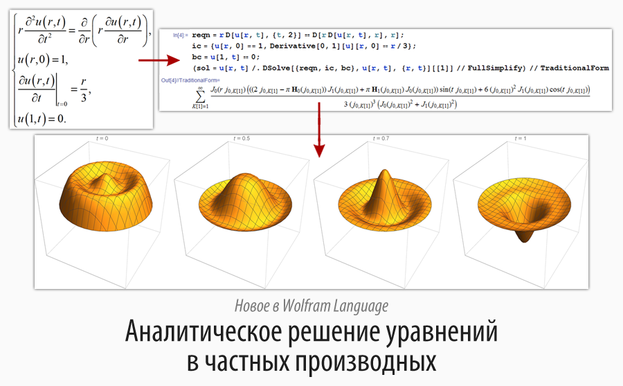
New in Wolfram Language | Analytical solution of partial differential equations

Translation of the post by Devendra Kapadia " New in the Wolfram Language: Symbolic PDEs ".
The code given in the article can be downloaded here .
I express my deep gratitude to Kirill Guzenko KirillGuzenko for his help in translating and preparing the publication .

---

Partial differential equations (PDE) play a very important role in mathematics and its applications. They can be used to simulate real phenomena, such as vibrations of a tensioned string, propagation of heat flux in the rod, in financial areas. The purpose of this article is to lift the curtain into the world of PDE (for those who are not familiar with it) and to acquaint the reader with how to solve PDC in Wolfram Language effectively using new functionality for solving boundary value problems in DSolve , as well as the new DEigensystem function, which appeared in version 10.3 .

The history of PDE goes back to the works of famous mathematicians of the eighteenth century - Euler, D'Alembert, Laplace, but the development of this field in the past three centuries has not stopped. And therefore in the article I will give both classical and modern examples of PDE, which will allow us to consider this area of ​​knowledge from different angles.

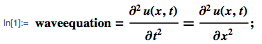
Let's begin by considering the vibrations of a tensioned string with a length of π fixed at both ends. String oscillations can be modeled using the one-dimensional wave equation given below. Here, u (x, t) is the vertical displacement of the point of the string with the x coordinate at time t :
')


Then we set the boundary conditions, thus indicating that the ends of the string retain their positions during vibrations.



We now define the initial conditions for the movement of the string, indicating the displacements and velocities of different points of the string at the moment of time t = 0 :



Now we can use DSolve to solve the wave equation with initial and boundary conditions:



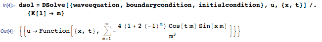
As stated above, the solution is an infinite sum of trigonometric functions. The amount is returned in an uncalculated form ( Inactive ), since each individual member of the expansion has a physical interpretation, and often even a small number of members can be a good approximation. For example, we can take the first four members to get an approximate solution asol (x, t)



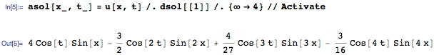
Each member adds up to a standing wave, which can be represented as follows:



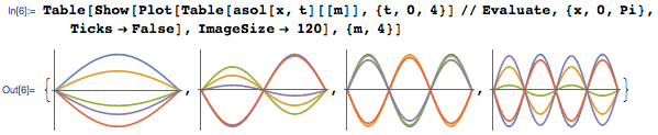
And all these standing waves fold together to form a smooth curve, as shown in the animation below:





The wave equation belongs to the class of linear hyperbolic partial differential equations describing the propagation of signals with finite velocities. This PDC is a convenient way to model oscillations in a string or in some other deformable body, but it plays an even more important role in modern physics and engineering applications, since it describes the propagation of light and electromagnetic waves.

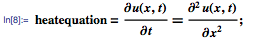
Let us now model the heat flux in a rod of unit length, isolated at both ends, using the following heat conduction equation:



Since the rod is insulated at both ends, a zero heat flux passes through them, which can be expressed as boundary conditions of the form x = 0 and x = 1:



Now you need to specify the initial temperature distribution in the rod. In this example, we will use the following linear function. In the left end (x = 0) the initial temperature is 20 degrees, in the right ( x = 1 ) it is 100:



And now we can solve the heat equation with given conditions:



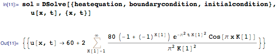
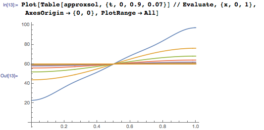
As in the above example with the wave equation, we can extract several terms of the sum and get an approximate solution:



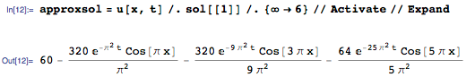
The first term of the approximate solution — 60 — is the average of the temperatures at the edges of the rod, and it is the stationary temperature for this rod. As shown in the graph of the temperature function from the length shown below, the core temperature quickly reaches a stationary value of 60 degrees:



The heat equation is a class of linear parabolic partial differential equations that describe diffusion processes. This seemingly simple equation can often be found in the most diverse and sometimes quite unexpected areas. Further in the article we will consider two examples of this phenomenon.

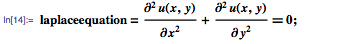
We now consider the Laplace equation, which is used to simulate the stationary state of systems, that is, the behavior after some time-dependent transient processes. In the two-dimensional case, this equation can be represented as follows:



Limit the x and y coordinates to the rectangular area Ω, as shown below:



The classical Dirichlet problem is to find a function u (x, y) satisfying the Laplace equation inside the domain Ω with a given Dirichlet condition ( DirichletCondition ), which determines the values ​​at the boundaries of the domain Ω, as shown below:



The Dirichlet problem can be solved using the DSolve function, while defining a very elegant area :



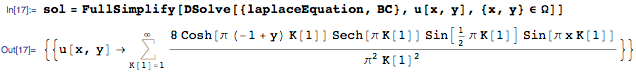
As in the examples earlier, we can extract a certain number of members (say, 100) from the sum and visualize the solution:



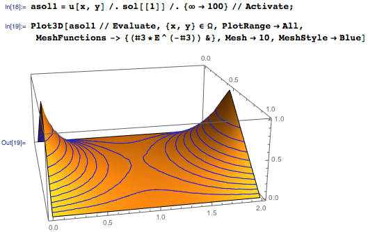
It should be noted that the solution u (x, y) of the Dirichlet problem seems smooth in Ω, despite the fact that the boundary conditions have sharp features. In addition, u (x, y) reaches extreme values ​​at the boundaries, while in the center of the rectangle is a saddle point. These features are characteristic of linear elliptic equations — a class of partial differential equations, to which the Laplace equation belongs.

The wave equation, the heat equation, the Laplace equation are the most famous examples of classical PDEs. Now we will look at three examples of typical modern PDCs, the first among which will be the Burgers equation for a viscous fluid, which can be represented as follows:



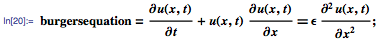
This nonlinear PDC was introduced by Johannes Burgers in the forties as a simple model for turbulent flows (the parameter ϵ in the equation is the viscosity of the fluid). However, ten years later, E. Hopf and D. Cole showed that the Burgers equation reduces to the heat equation, which means that this equation cannot exhibit chaotic behavior. The Cole-Hopf transformation allows us to solve Burgers equations in a closed form for the initial condition given, for example, as follows:



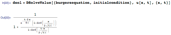
In this example, we will use the DSolveValue function , which returns only the expression for the solution. The terms with the error function ( Erf ) in the formula below arise from the solution of the corresponding boundary value problem of the thermal equation:



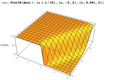
The graph below shows the time variation of a hypothetical one-dimensional flow velocity field. The solution seems smooth for positive ϵ, while the initial condition is a piecewise given function:



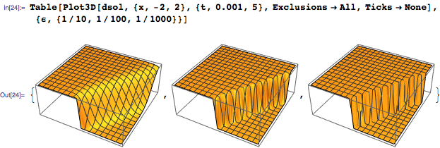
As can be seen in the graphs below, the solution tends to be discontinuous when viscosity tends to zero. Such solutions with a sharp transition (shock solutions) are a well-known feature of the Burgers equations for non-viscous (ϵ = 0) media.



As a second example of modern PDCs, consider the Black-Scholes equation used in financial calculations. This equation was first introduced by Fisher Black and Myron Scholes in 1973 as a model for determining the theoretical price of European options, and it is formulated as follows:



Where:
c is the price of the option as a function of the value of shares s and time t,
r - interest rate without risk,
σ - stock volatility.

In their landmark article (which was cited more than 28,000 times), Black and Scholes noted that their equations can be reduced to the heat equation by transforming variables. This drastic simplification leads to the famous Black-Scholes formula for European options with final conditions based on the strike price of the asset at time t = T:



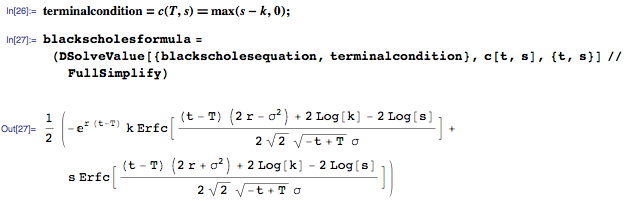
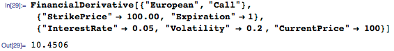
Armed with this formula, we can calculate financial option values ​​for typical parameter values:



The answer is consistent with the value obtained using the built-in function FinancialDerivative :



As the third example of modern PDCs, we consider the Schrödinger equation for an electron in a one-dimensional potential well with a depth d and the corresponding initial condition. The equation and conditions can be formulated as follows:



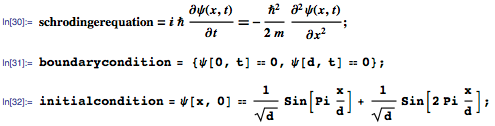
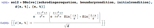
This example has an elementary solution that takes imaginary values ​​due to the presence of I in the Schrödinger equation:



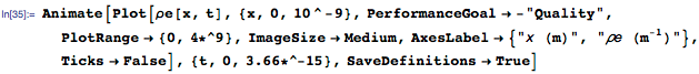
The probability density function for the electron ρ = Ψ ^⊹ Ψ, using the appropriate values ​​of the parameters in the problem, can be calculated as follows:



We can create an animation of the change in probability density over time, which shows that the "center" of the electron in the well moves from side to side:





Eigenvalues ​​and eigenfunctions play an important role both in solving the Schrödinger equation and in other PDEs. In particular, they provide “building blocks” for solving wave equations and heat conduction equations in the form of infinite sums, which were cited earlier in the article. Therefore, as our last example, we consider the problem of finding the nine smallest eigenvalues ​​and eigenfunctions for the Laplace operator with the homogeneous (zero) Dirichlet condition for a three-dimensional spherical region. Let us find the nine smallest values ​​of λ and the corresponding functions ϕ satisfying Λϕ = λ ϕ, which are defined as follows:



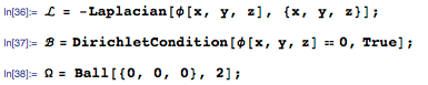
The new function DEigensystem in version 10.3 allows you to calculate the required eigenvalues ​​and functions as follows:



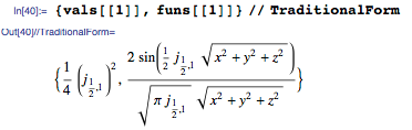
The eigenvalues ​​in this problem are expressed in terms of BesselJZero . Here is an example:



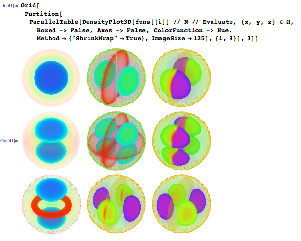
Eigenvalues can be visualized using the DensityPlot3D function , which returns beautiful graphs, as shown below:



PDE are an important tool in many branches of science and technology, statistics and finance. At a more fundamental level, they provide exact mathematical formulations of some of the most profound and delicate questions about our Universe, say, about the possibility of the existence of bare singularities . In my experience, studying PDEs rewards with a rare combination of practical ideas and intellectual satisfaction.

I recommend to study the documentation on DSolve , NDSolve , DEigensystem , NDEigensystem and the finite element method to learn more about the different approaches to solving PDE in Wolfram Language.

The PDA is symbolically supported in Wolfram Mathematica and Wolfram Language from version 10.3, and will soon be presented in all other Wolfram software products.