Digital filtering on FPGA - Part 2

Hello!
This is the second publication on the topic “Digital filtering on FPGA”. The second part will be devoted to the practical implementation of FIR filters on FPGAs. In the process of preparing the material, I realized that it would swell to unprecedented sizes, but I did not want to divide it into several parts. Therefore, all the subtleties of the theory and synthesis of FIR filters will be in one article, divided into interrelated sections. I will begin the review with the theoretical part, in particular, I will tell you about the features and methods of calculating the filter coefficients. Consider in detail the creation of FIR filters in various environments - MATLAB, CoreGENERATOR, Vivado HLS. All interested in asking under the cat.
Part 2. FIR filter
Theory
Consider a simple example of implementing FIR filters. As is known, there are two large classes of filters - IIR, with infinite impulse response and FIR, with finite impulse response . Let us dwell on the second type: FIR filters (FIR - “finite impulse response”). An FIR filter is a linear digital filter whose main feature is its time-limited impulse response, that is, from a certain point in time it becomes zero. As a rule, most FIR filters are executed without feedback, therefore almost all FIR filters are non-recursive.
')
This is how the implementation of the FIR filter looks in general, in particular - on the FPGA.
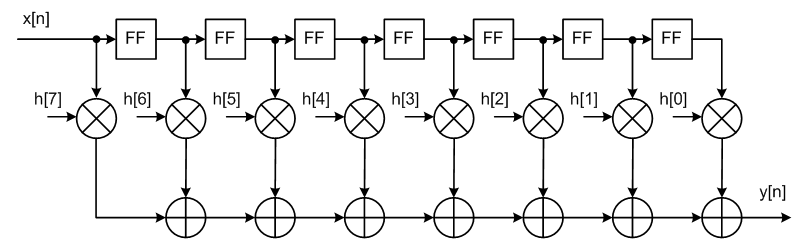
All FIR filters are described by the following equations:

where y (n) is the output signal (function of the current and past values at the input), x (n) is the input action, h (k) is the impulse response coefficients, N is the filter length (the number of filter coefficients), H (z) is filter transfer characteristic.
What is the secret of FIR filters?
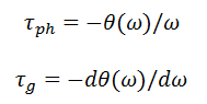
The most important feature of FIR filters is the ability to obtain accurate linear phase response . The reader has a logical question - “why is this necessary?”. Let us dwell on this moment in more detail. The signal undergoes various transformations as it passes through the filter. In particular, the amplitude and phase of the signal vary depending on the frequency response of the filter (amplitude, frequency response and phase, phase response). For multi-frequency signals, it is unacceptable that during the passage of processing units, the phase of the signal is distorted. Moreover, if the frequency response in the passband is practically constant, then there are problems with the phase response. To estimate phase distortions, it is convenient to introduce the concepts of phase and group delays.
The phase delay is the amount of delay for each of the frequency components of the signal. Defined as the phase angle divided by the frequency. Group delay is the average time delay of the entire multi-frequency signal. It is defined as the phase derivative with respect to frequency. Mathematically, phase and group delays are written as follows:
From the formula for group delay, the linearity condition of the phase response filter becomes obvious. If the phase response is linear, then the group delay after taking the derivative is equal to a constant, that is, constant for all frequency components. It is logical that the filter with nonlinear frequency response will introduce distortion in the phase of the signal.
Thus, the linearity of the phase response is one of the most important features of FIR filters. Let us dwell on the study of this class of filters.
FIR filters with linear phase response
To ensure the linearity of the phase response, the symmetry condition of the impulse response (or coefficients) of the filter must be met. Simply put, the FIR filter with linear phase response is symmetric. There are 4 types of filters that differ in the parity of the order of the filter N and the type of symmetry (positive or negative). For example, for filters with negative symmetry, a phase shift of 90 ° can be obtained. Such filters are used to design differentiators and the Hilbert transform. The impulse response curve of the FIR filter is constructed according to the ~ sin (x) / x law, regardless of the type of filter (low pass filter, high pass filter, PF, RF, differentiator). To solve practical problems, it is often not necessary to think about what type of filter is chosen. I will not give the proof of the condition of symmetry of the coefficients, but a curious reader can find it himself in various literature, the links to which I cite at the end of the article.
Designing FIR filters
The “calculation of the FIR filter” in most cases means the search for its coefficients by the values of the frequency response. I can not recall cases when the inverse problem would be solved with the exception of academic interest.
When creating a new digital FIR filter, any engineer goes through certain stages of development *:
- Filter specification Sets the filter type (low pass filter, high pass filter, band pass, notch), the number of N coefficients, the required frequency response, with tolerances for nonlinearity in the attenuation band and the passband, and so on.
- The calculation of the coefficients . By any available means and methods, filter coefficients are computed that satisfy the specifications from the previous paragraph.
- Analysis of the consequences of a finite bit depth . At this stage, the effect of quantization effects on the filter coefficients, intermediate and output data is evaluated.
- Implementation . At this stage, a filter is developed in an accessible programming language or the filter is implemented by creating ready-made IP cores.
* - development stages may be somewhat different, but the essence is always the same.
Filter specification
At this stage, the engineer searches for compromise solutions for implementing the required filter with the necessary parameters. There are not many of them, but one often has to sacrifice one parameter in order to achieve the required values in other quantities.
- Apass - bandwidth irregularity,
- Astop - attenuation level in the suppression band,
- Fpass - bandwidth cutoff frequency
- Fstop - the limiting frequency of the attenuation band,
- N is the order of the filter (the number of filter coefficients).
In practice, the Apass and Astop parameters are set in decibels (dB), and the distance between Fpass and Fstop expresses the width of the filter transition band. It is logical that the value of Apass should be as low as possible, Apass as much as possible, and the ratio Fpass / Fstop ideally tends to one (perfectly rectangular frequency response). The number of coefficients is not in vain entered into the filter specification. As will be shown later, the parameters of the frequency response of the filter, as well as the amount of FPGA resources, depend on the order of the filter N and the width of the coefficients.
Calculation of filter coefficients
You can write several books and scientific articles on this topic, but in this article we will not consider in detail all the methods. There are many methods for calculating filter coefficients - the method of weighting by window functions, the method of frequency sampling, various optimal (according to Chebyshev) methods using the Remez algorithm, etc. All methods are unique in their characteristics and give some results. For the windowing method, the Gibbs effect , which introduces non-uniformity and outliers into the frequency response of the filter between the calculated points of the function, becomes a negative manifestation. You can fight it endlessly, but in practice they introduce tolerances for irregularities in the passband and suppression band.
The main method for calculating coefficients for many filters is the modified Remez algorithm, the Parks-McClellan algorithm . At its core, it is an indirect iterative method for finding optimal values with a Chebyshev filter characteristic. A feature of the method is to minimize errors in the attenuation and transmission band by the Chebyshev approximation of the impulse response. It is logical that the greater the number of coefficients, the smaller the non-uniformity of the frequency response and the more rectangular it is.
The final result depends on the choice of method, but they all boil down to the same goals - minimizing emissions in the passband and increasing the “squareness” of the frequency response.
Final Impact Analysis
The width of the coefficients - the main factor on which depends the type of frequency response. In modern FPGAs, the width of the coefficients can be chosen any, but reasonable numbers lie in the range from 16 to 27 bits. For high filter orders, it is often required to provide a large dynamic range of the discharge grid, but if this cannot be done, sooner or later quantization errors begin to appear. Because of the limited bitness of the coefficients, the frequency response is modified, and in some cases it is distorted so much that you have to sacrifice the parameters from the frequency specification to achieve an acceptable result. Anyway, the bitness of the representation of the coefficients directly affects the maximum possible attenuation of Astop. Therefore, when using a too limited bit grid of coefficients, it is sometimes impossible to achieve the desired suppression even with huge filter orders!
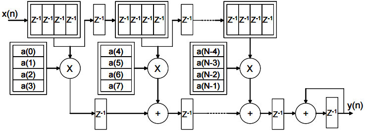
The bit length of the intermediate data and the arithmetic overflow are factors that also determine the type of frequency response and the result at the filter output. In many FPGAs, the problem is eliminated using high-capacity batteries in DSP units. For example, in the FPGA Xilinx 6 and 7 series in the cells of DSP48E1 48-bit batteries and multipliers are used. The following figure shows the standard DSP48E1 unit on which FIR filters are implemented.

The built-in DSP blocks of modern FPGAs are designed in such a way as to most conveniently carry out DSP tasks. First of all - to implement FIR filters.
Implementation
To implement the simplest filters, very few logical operations are required. The main node with which the FIR filter is implemented is the FPGA DSP block. All mathematical operations occur in this block - multiplication of input samples with filter coefficients, input signal delay, data summation. Modern DSP nodes contain a preliminary adder, so even the summation operations for filters with a symmetrical EI can be done inside this node. In addition to the DSP block, the filter needs memory to store the coefficients (distributed or block). More filter does not use anything. The figure shows the implementation of an FIR filter using multipliers, batteries, delay lines, and memory for storing coefficients.
Calculation of the filter in MATLAB
There are many applications in which you can calculate the filter and search for its coefficients. For example, LABView, Scope FIR, FDATool from MATLAB or the free analogue of Octave. Perhaps the most convenient means of calculating the FIR filter is MATLAB. To run the filter creation and analysis tool, you need to type the keyword fdatool in the environment command window. A window like this will appear (depending on the version of MATLAB, it may have a slightly different look):
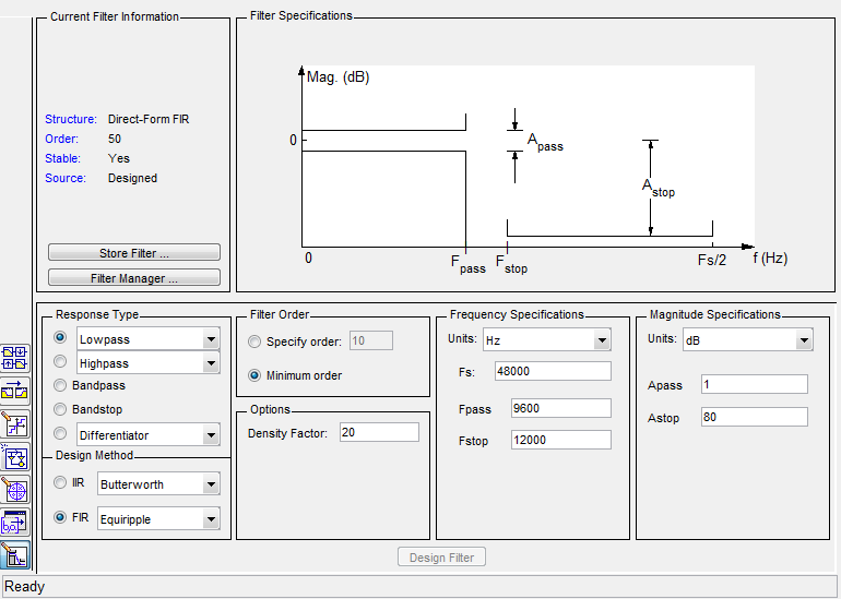
The main parameters are set in the Filter Specifications window. Depending on the filter settings, certain parameters may appear in the main window area.
- Filter Order - determines the filter order (minimum or user-defined) **.
- Frequency Specifications - defines the frequency parameters of the filter characteristics.
- Magnitude Specifications - defines the amplitude parameters of the filter characteristics.
- Density Factor - for Equiripple type, sets the grid of points by which the frequency response of the filter is approximated.
** - in FDATool, the order of the filter N is one more than the specified one (if you set N = 7, then the utility calculates 8 coefficients) !!!
Response type - the type of the transfer characteristic of the filter. In this field, select any filter that exists in nature, for example:
- Lowpass - low pass filter,
- Raised cosine - raised cosine filter,
- Highpass - high pass filter,
- Bandpass - bandpass filter
- Bandstop - notch (blocking) filter,
- Differentiator - differentiator,
- Nyquist - Nyquist filter,
- Multiband - multiband filter,
- Hilbert transformer - Hilbert's converter,
- Arbitrary magnitude - filters with arbitrary frequency response.
Moreover, depending on the type of filter, the analysis tool will indicate restrictions on the type of filter and will offer to enter the correct value of N.
Design Method — selects the filter design method and its type (IIR or FIR). Available options for IIR filters:
- Butterworth - filters with Butterworth characteristic,
- Chebyshev Type I, II - Chebyshev filters,
- Elliptic - elliptic filter,
- Maximally flat - a filter with the most flat response in the passband,
For FIR filters are available options ***:
- Equiripple - a filter with a uniformly pulsating frequency response,
- Least-squares - least squares filter,
- Window - window-weighted filter with various functions ****,
- Complex Equiripple - complex filter with uniformly pulsating frequency response,
- Maximally flat - a filter with the most flat response in the passband,
*** - Equiripple and Window filters are of the greatest practical interest.
**** - when this option is selected, an access panel to window functions and their parameters appears.
For the Equiripple method, the simplest calculation of an FIR filter is performed using a modified Remez algorithm. The user sets the parameters from the specification for the filter and immediately sees the result. In the case of unsatisfactory results, you can change one or several filter parameters at any time and get another frequency response. The calculation is carried out until the required characteristics are obtained. If it was not possible to achieve the values for the task, then sooner or later it will be necessary to sacrifice one or another value from the specification, or significantly increase the order of the filter N.
Several window functions are available for the Window method: Bartlett, Blackman, Blackman-Harris, Chebyshev, Flat Top, Gaussian, Hamming, Hann, Kaiser, Rectangular , etc., up to user-defined window functions (User-defined). All these functions have their own characteristics and can give different parameters of the frequency response of the FIR filter. Some window functions are calculated without parameters, and some filters are set through certain parameters affecting the frequency response of the filter.
Of all the window functions presented, in my opinion, the Kaiser window is the most convenient. To build the frequency response, you only need to set one Beta parameter, which affects the level of suppression in the attenuation band and the squareness of the frequency response.
At the bottom left of the main working area, the FDATool tool contains additional tabs in which you can specify the filter type (decimator or interpolator), the name of the model to insert into Simulink, the type and length of the coefficients and input data, and much more. For practical purposes, the most basic tabs are Design Filter — it calculates the filter, and Quantinization Parameters — in this tab, you can specify the type and bitness of the data.
On the top panel there are buttons with which you can view the frequency response and phase response of the filter, group and phase delay, pulse and transient characteristics, a map of filter zeros and poles, calculated coefficients, etc.
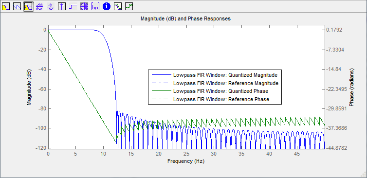
Screenshots of the FDATool workspace
Graph of frequency response and phase response of the filter:
Graph of the impulse response of the filter:

Chart of zeros and poles:

Graph of the impulse response of the filter:
Chart of zeros and poles:
In addition to all this, FDATool allows you to import and export filter models and calculated coefficients. For example, you can calculate a filter and send its model to Simulink as a model on standard primitives. You can calculate the coefficients and save them in a separate file, for example, as a file with the extension * .h (header).
Header file * .h with filter coefficients
/* * Discrete-Time FIR Filter (real) * ------------------------------- * Filter Structure : Direct-Form FIR * Filter Length : 128 * Stable : Yes * Linear Phase : Yes (Type 2) * Arithmetic : fixed * Numerator : s16,15 -> [-1 1) * Round Mode : convergent */ /* General type conversion for MATLAB generated C-code */ #include "tmwtypes.h" const int BL = 128; const int16_T B[128] = { -18, 0, 19, 39, 58, 75, 88, 97, 100, 96, 85, 68, 44, 16, -16, -50, -83, -113, -139, -157, -166, -164, -152, -128, -94, -51, 0, 55, 111, 164, 211, 248, 272, 280, 269, 240, 192, 126, 45, -47, -146, -245, -339, -421, -483, -521, -528, -501, -434, -329, -183, 0, 217, 462, 728, 1006, 1288, 1564, 1823, 2056, 2254, 2409, 2517, 2571, 2571, 2517, 2409, 2254, 2056, 1823, 1564, 1288, 1006, 728, 462, 217, 0, -183, -329, -434, -501, -528, -521, -483, -421, -339, -245, -146, -47, 45, 126, 192, 240, 269, 280, 272, 248, 211, 164, 111, 55, 0, -51, -94, -128, -152, -164, -166, -157, -139, -113, -83, -50, -16, 16, 44, 68, 85, 96, 100, 97, 88, 75, 58, 39, 19, 0, -18 }; In addition, you can create a coefficient file * .COE in a special format for Xilinx. To do this, select the type of coefficients with a fixed point and set their width. Then click Targets -> Xilinx Coefficient (.COE) File , as a result of which the contents of the file are displayed in the main MATLAB window - global settings and coefficients in HEX format.
Example * .coe file
; XILINX CORE Generator(tm)Distributed Arithmetic FIR filter coefficient (.COE) File ; Generated by MATLAB(R) 8.3 and the DSP System Toolbox 8.6. ; ; Generated on: 06-Dec-2015 15:35:35 ; Radix = 16; Coefficient_Width = 18; CoefData = 3ffeb, 00018, 00049, 00067, 0005f, 00029, 3ffd2, 3ff79, 3ff46, 3ff59, ... It is seen that when a single impulse is fed to the input, nothing else is formed at the output, as the filter impulse response (graph from Simulink).

Xilinx FIR Compiler
As in the case of the CIC filter, I will provide a detailed description of the means for creating FIR filters from Xilinx. I note that the description contains not just a translation from a datasheet, but comments and recommendations from the personal experience and experience of my colleagues.
FIR Compiler - Tab 1:
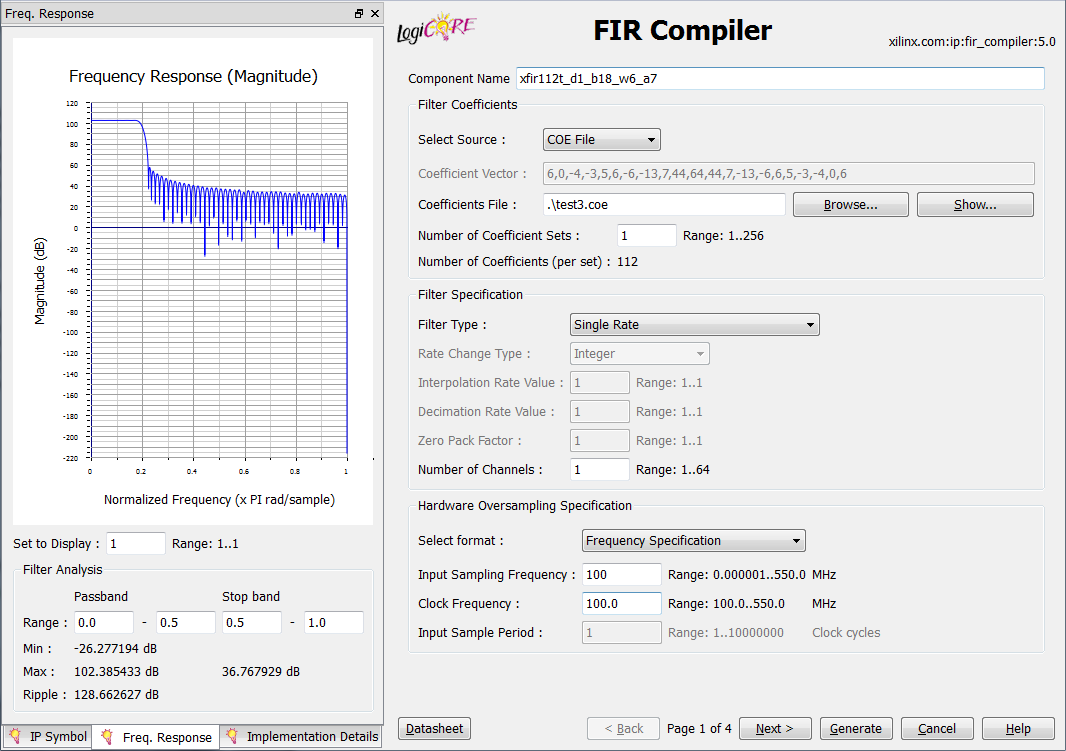
Component name - the name of the component (the Latin letters az, the numbers 0-9 and the symbol "_" are used).
I recommend using meaningful names in which the main filter parameters are encrypted. For example, xfir128t_d1_b18_4c_w6_a7 is a filter made for Xilinx, N = 128 (taps), decimation is not used, the width of the coefficients is 18, four channels, the Kaiser window function with the parameter beta = 6, the FPGA chip is Artix-7.
Filter Coefficients:
- Select source - select the source of the coefficients ( Vector - a vector specified manually or COE File - a file with a set of coefficients). It is preferable to use overloaded * .COE files.
- Coefficient Vector - a vector of coefficients set by hand.
- Coefficient File is a vector of coefficients read from a file.
- Number of Coefficient Sets - the number of actually used DSP blocks for processing coefficients. The number of coefficients must be divided completely by the specified value. A useful option when operating at a high frequency relative to the sampling frequency, allows you to significantly save FPGA resources.
- Number of Coefficient (per set) - the number of coefficients processed at a time by DSP blocks. The value in the field is automatically set when reading the number of coefficients and the previous parameter.
Filter Specification:
- Filter type - filter type: simple / interpolating / decimator / polyphase.
- Rate Change Type - change processing speed. May be integer or fractional.
- Interpolation / Decimation Rate Value - interpolation / decimation coefficient.
- Zero Pack Factor - for interpolating filters, the parameter determines the number of zeros inserted between the coefficients.
- Number of channels - the number of independent filtering channels: 1-64.
Hardware Oversampling Specification: These parameters affect the output sampling rate, the number of cycles required for data processing. The level of parallelism within the kernel and the amount of resources occupied also depend on these parameters.
- Select format - selects the frequency ratio of the filter: Frequency Specification / Sample period.
- Frequency Specification - Frequency specification: the user sets the sampling rate and the frequency of data processing.
- Sample period - Clock specification: the user sets the ratio of the processing frequency to the clock frequency of the data.
- Input Sampling Frequency - input sampling rate: *.
- Clock frequency - filter processing frequency: *****.
- Input Sampling period - the ratio of the processing frequency to the frequency of the input clock signal: *****.
***** - the range depends on the general settings and the sampling rate R.
FIR Compiler - Tab 2:
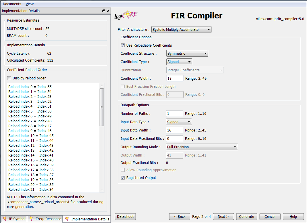
Filter Architecture - sets the implemented architecture of the filter.
- Systolic Multiply Accumulate - an accumulated systolic filter,
- Transpose Multiply Accumulate - tunable filter with accumulation,
- Distributed Arithmetic - filter on FPGA distributed logic.
Coefficient Options - parameters for coefficients
- Use Reloadable Coeffcients - use reloadable coefficients. Useful option to implement in one filter overload frequency characteristics.
- Coefficient Structure - structure of coefficients, 5 types: asymmetric, symmetric, negatively symmetric, half-strip and with the Hilbert transform. By default, the FIR compiler tries to determine the type of coefficients (inferred).
- Coefficient Type - type of coefficients: signed or unsigned.
- Quantization - sets the rounding method: integer coefficients, rounding to the nearest integer or maximum dynamic range (scales the coefficients relative to the maximum).
- Coefficient Width - the width of the coefficients. The value in this field affects the frequency response of the filter, which can be observed in the corresponding window (Freq. Response).
- Best Precision Fraction Length - automatically sets the best ratio for the whole and fractional parts of the discharge grid.
- Coefficient Fractional Bits - defines the position for separating the whole part from the fractional in the bit grid of the coefficients representation.
Datapath Options - input options
- Number of Paths - determines the number of parallel channels for processing. The number of DSP cores is proportional to the value in this field. For this option, several independent data streams are input to the filter, while for the Number of Channels parameter, the data is received at one input and processed sequentially.
- Input Data Type - data type at the input of the filter (signed or unsigned).
- Input Data Width - the width of the input data.
- Input Data Fractional Bits - determines the number of bits per fractional part of the input data representation. The value in this field does not affect the implementation of the filter! (a fixed-point number can be represented as you please: with a fractional part or without it, but the result is the same).
- Output Rounding Mode - output rounding mode: full precision, discarding the least significant bits, rounding to the whole up / down, rounding to even / odd. In many tasks, this parameter is not required to change and you can leave Full Precision - full accuracy.
- Output Width - the width of the output filter.
- Output Fractional Bits - the number of bits that define the fractional part of the output. The field is informative and does not affect the implementation of the filter.
- Allow Rounding Approximation - for Symmetric Rounding Mode, the option allows approximation when rounding without additional resource costs (automatic determination of the sign bit in a word).
- Registered Output - the active option adds an additional register to the filter output to increase the performance (maximum processing frequency) of the filter.
FIR Compiler - Tab 3:
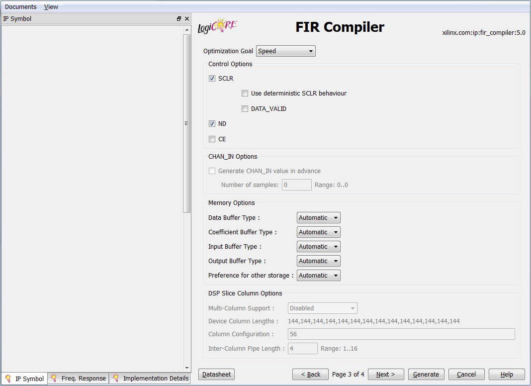
Optimization Goal - defines the optimization goal when creating a filter (Area - by area, Speed - by speed). In most cases, it is possible to simultaneously achieve maximum speed and minimum resource expenditures, but in specific cases, when specifying Speed, the filter optimally places the internal registers in the critical paths between logical functions.
- SCLR - synchronous filter reset (a logical unit at the input resets).
- Use Deterministic SCLR Behavior - defines the behavior of the internal data of the Multiply-Accumulate filter type during the reset process. With the active option, the reset signal clears the internal registers, data memory and storage coefficients.
- ND - "New data", the input signal that determines the flow of data to the input of the filter. Together with the RFD signal allow you to organize batch processing. As a rule, the ND and RFD signals are connected to the control signals of the FIFO.
- CE - “Clock Enable”, filter enable signal. At a low level at the input of this signal, any processing inside the filter is suspended, regardless of whether new data arrive or not.
- DATA_VALID - signal of validity of the output data. This option is useful only in multi-channel mode (Number of Channels> 1).
Memory Options - global settings for selecting the type of memory for storing input data, filter coefficients, intermediate and output data. Choosing block memory instead of distributed memory, in some cases, you can save logical FPGA resources hundreds of times!
For Data / Coefficient / Input / Output Buffer Type, Auto / Block / Distributed modes are possible.
Preference for Other Storage - defines the type of memory for intermediate data. Also available modes are Auto / Block / Distributed.
DSP Slice Column Options - defines the settings for the distribution of DSP blocks between the FPGA columns. For some filter architectures, for example, with symmetric coefficients, Multi-Colomn Support mode is not available, so you need to monitor the possible implementation of the filter.
- Device Column Lengths - determines the length of the columns of DSP blocks. Useful informative field in which you can pre-define the upper limit of the order of the filter and the maximum number of implemented filters.
- Column Configuration - determines the configuration and position of DSP blocks in columns. It is necessary to work with this parameter carefully, since a large delay may occur when the filter is broken between several columns, therefore the maximum clock frequency will drop.
- Inter-column Pipe Length - determines the number of additional registers between columns of DSP blocks to eliminate the negative effect of the propagation delay.
FIR Compiler - Tab 4:
Summary - this tab in the form of a list reflects the final filter settings (number of channels, filter order, frequency parameters, input, output and intermediate data width, coefficient width, filter delay, number of DSP blocks used, presence of control signals, etc.) .
On the left side of the FIR Compiler window there are three useful additional tabs:
- IP-symbol - a schematic view of an IP block with active I / O ports.
- Freq. response - frequency response of the FIR filter.
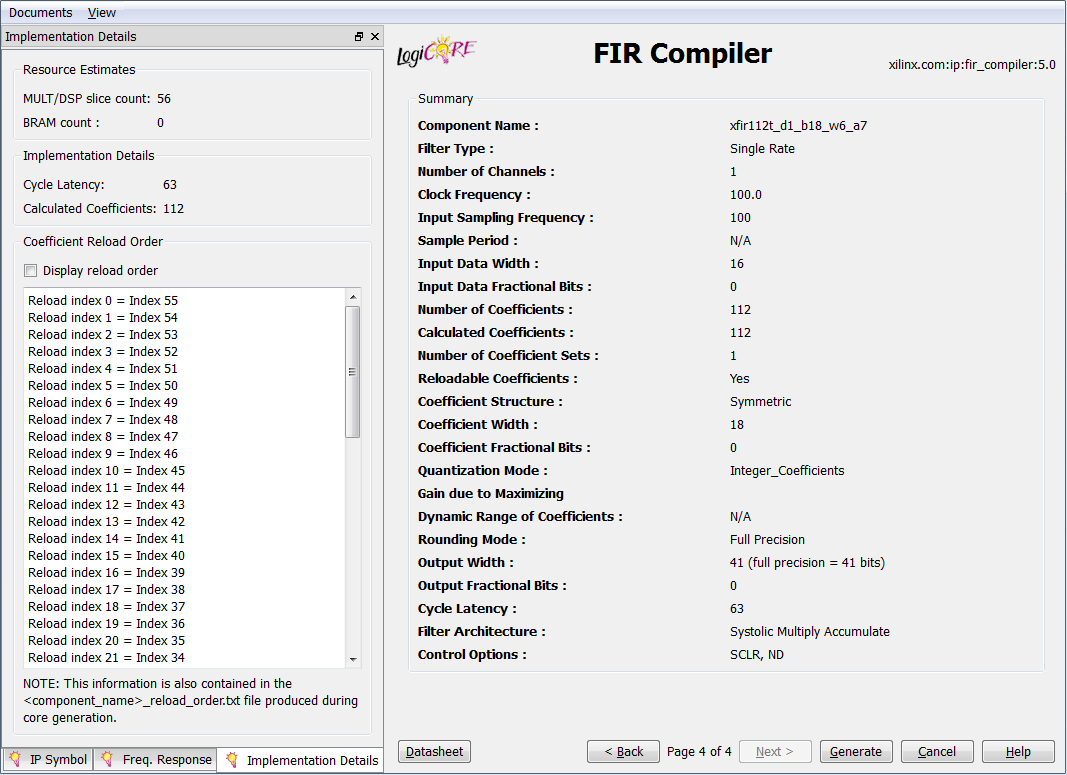
- Implementation Details - an estimate of the occupied resources of the DSP and RAMB, the total delay, the number of coefficients and the order of their loading.
Abstract example
Condition
We will calculate the wideband preprocessing filter with the following parameters:
- Fs sampling rate: 250 MHz,
- Fpass filter cutoff frequency: 55 MHz
- Squareness coefficient:> 0.88 (Fpass / Fstop),
- Bandwidth Suppression (Apass): <0.5 dB,
- Attenuation in the attenuation band (Astop):> 50 dB.
Decision
Step 1: FPGA Resource Assessment
You need to understand how much crystal resources are available to implement such a filter. In the DS180, you can find that the chip has 240 DSP48E1 blocks arranged in three columns (this is important!). It is known from TZ that the EM is symmetrical, which means that the filter of order N will require N / 2 blocks DSP48E1. Therefore, on the selected chip, it is possible to implement 2 filters with a characteristic length of N = 240, or 6 filters with a length of N = 80. For practical purposes, when processing signals, the length of the EM is chosen to be a multiple of the power of two. For example, N = 64, 128, or 256. Or, N = (128 + 64), (32 + 16 + 8). In our case, it is necessary to implement 6 filters on 240 DSP blocks. Given the symmetry for each filter, it is possible to use a length of N <81 coefficients. Suppose that to achieve the filter parameters N = 80 = 64 + 16 coefficients suffice.
Step 2: Find Filter Ratios
Run FDATool and enter the filter parameters from the specification into the required fields (remember that the order of N is set to 1 less than the true order of the filter). Mode 1 - Equiripple . For the cutoff frequency Fpass = 55 MHz and squareness ratio> 0.85, we find the barrier frequency Fstop <62.5 MHz. The following figure shows the calculation of the filter according to the required parameters:
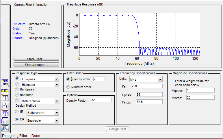
As you can see, the filter satisfies all the listed requirements.
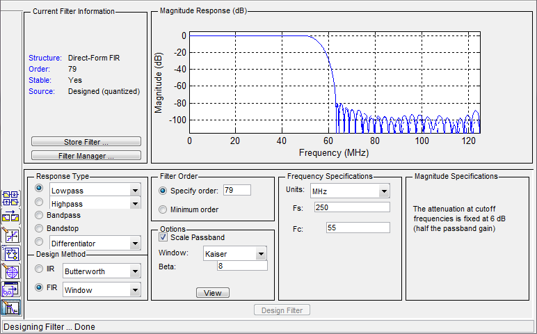
Mode 2 - Window . Suddenly, just before the delivery of the project, your abstruse customer got a thought in his head. “I want 70 dB suppression, all other things being equal!” The element base is selected, the board is divorced and assembled, the FPGA is installed, the project has been debugged for several months and there is no possibility to deliver something to redo. What to do? Design your own FIR filter a week before the project is completed? Search for other methods of suppressing the frequency response? Redo the board and install FPGA fatter? Unreal! The main thing - do not panic. Equiripple method does not save. Go to the window mode Window. When choosing my favorite Kaiser window, you can achieve better filter performance. For example, to provide the necessary suppression in the attenuation band Astop = 80 dB (parameter Beta = 8). But for the window method, one should take into account that in the attenuation band, quantization effects can manifest themselves in the decay band because of the insufficient bitness of the coefficients.
Further, in a known manner, upload the calculated coefficients to the * .COE file for further work.
Step 3: Implementation
The number of channels and coefficients was chosen in such a way that the DSP48E1 resources in the FPGA are 100% occupied. The number of occupied resources for 6 channels in the figure below:
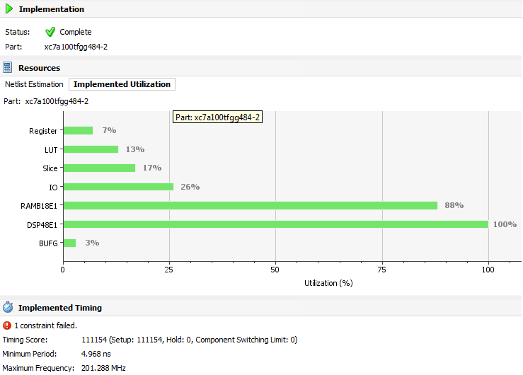
Do not be afraid that the project will not work at 250 MHz. How it will work. PlanAhead loves to be reinsured and indicates values below real. The results of the wiring of six channels FIR filters.
Beautiful drawings layout project
Schematic view of the part of the IP kernel FIR filter:

PCB layout in FPGA Editor (Zoom bottom):
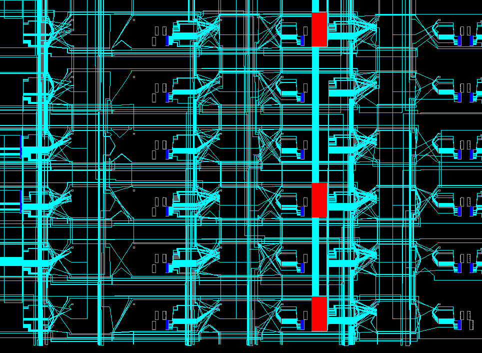
Board layout in FPGA Editor:
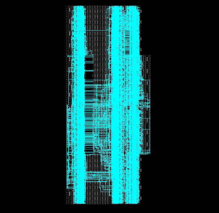
PCB layout in FPGA Editor (Zoom bottom):
Board layout in FPGA Editor:
Practical advice
Of course, the transition to the Window does not always save, and in practice there are several other methods that somehow simplify the life of the developer.
- Determine in advance the possible decimation of the signal (with respect to the sampling frequency and the cut-off frequency in the signal spectrum). Use cheap CIC filters for decimation. After decimation, it is possible to reduce the number of DSP blocks used by the crystal.
- Determine the ratio of the sampling rate and the processing frequency in the FPGA chip. If the processing frequency is several times higher than the sampling rate, you can save the same amount of resources by the FIR filter implementation.
- Implement the filter on the distributed logic of the FPGA, if it is possible and not critical from the point of view of processing frequencies. This method is very difficult to implement and will not work stably for large orders of the filter N.
- To implement filters with symmetric IC, it is preliminary to estimate the size of the columns of DSP blocks and the number of these columns in the FPGA. To implement long filters with a symmetric IC, a cascade connection of DSP blocks is required and when placing the filter inside the FPGA in one column, the DSP cells may not be enough. On the other hand, when implementing independent filter channels, there may simply not be enough columns if only one filter can fit in each column. It is necessary either to reduce the length of the characteristic, or to make two small filters with a smaller number of coefficients. ******
- For modern FPGA crystals (Altera and Xilinx), when implementing a filter with a symmetric EM, use a preliminary adder in the DSP node, and not on distributed logic. An internal pre-adder saves not only logical cells, but also crystal trace resources! *******
******* - for FPGA chips manufactured by Xilinx 7 series and older, this method saves only if the digit capacity of the coefficients does not exceed 18. For Uber-modern as of 2015-2016, Xilinx Ultra-Scale chips are possible implement a preliminary adder with a coefficient of 24 coefficients.
Vivado hls
Modern methods for creating nodes tasks of digital signal processing on the FPGA are reduced to two principles:
- reduction of design time (the concept of " time-to-market "),
- reduction of the entry threshold (popularization of FPGA among C ++ developers).
Both principles did not come about by chance and are primarily due to the constant increase in the logical capacity of the FPGA. Xilinx declares that the old programming methods (in VHDL and Verilog) no longer cope with modern tasks, and there is a high probability that in the future programming on FPGA will be conducted exclusively in high-level languages such as C and C ++. Xilinx a few years ago announced a new design tool called Vivado HLS and offers all large projects to partially or fully transfer to a new level. Development on Vivado HLS is reduced to the fact that you can get away from the concept of " clock frequency " and develop complex algorithms without reference to the FPGA, and all the optimization under the FPGA is already done at the last stage of the project. Let's see what can be done with the help of the new environment and develop the simplest FIR filter in Vivado HLS.
As an example, I took one of the labs from Xilinx, in which, as a first approximation, all the power of modern tools is shown. The main development with the help of Vivado HLS is based on interrelated tasks: writing code and optimizing it for speed (Speed) and occupied area (Area) with the help of directives.
Xilinx proposes the following design behavior:
- - C Validation / Simulation ( Project -> Run C Simulation ): writing an algorithm, debugging a project, identifying errors in the code, comparing data with a standard, etc.
- - C Synthesis ( Solution -> Run C Synthesis ): project synthesis from C-code to RTL form and analysis of the received data: performance evaluation (latency, trip count, speed etc.), resource estimation, received input / output interface. *
- - RTL Verification ( Solution -> Run C / RTL Cosimulation ): reuse the C-model of the main () test to analyze the RTL model (self-checking).
- - IP Creation ( Solution -> Export RTL ): creation of an IP core for further use in the main project (Xilinx ISE, Vivado, etc.)
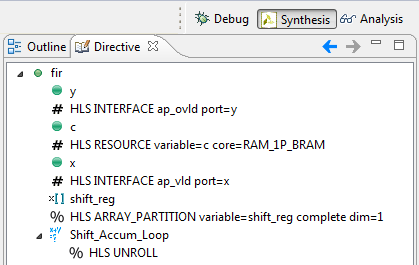
How to make different decisions? Use directives is a tool for optimizing projects in Vivado HLS.Directives can be added to the source code ( Source file ) or to a separate directive file .
- Source file - suitable for setting directives that WILL NOT be changed during project creation. For example, the directives for the interface ports I / O do not change. In the draft, these directives are indicated by the prefix: #HLS .
- Directive file - suitable for setting conditions and constraints that affect speed and placement optimization. As a rule, a project can compare several solutions in different solutions and choose the optimal one. In the project, these directives are indicated by the prefix: % HLS .
I will give an example of the source for the simplest FIR filter. Pay attention to the directives in the source code.
FIR Filter C ++ for Vivado HLS
#include "fir.h" void fir ( data_t *y, coef_t c[N], data_t x ) { <b>#pragma HLS</b> INTERFACE ap_ovld port=y <b>#pragma HLS</b> INTERFACE ap_vld port=x <b>#pragma HLS</b> RESOURCE variable=c core=RAM_1P_BRAM static data_t shift_reg[N]; acc_t acc; data_t data; int i; acc=0; Shift_Accum_Loop: for (i=N-1;i>=0;i--) { if (i==0) { shift_reg[0]=x; data = x; } else { shift_reg[i]=shift_reg[i-1]; data = shift_reg[i]; } acc+=data*c[i];; } *y=acc; } Directives in a separate file are as follows:
set_directive_unroll "fir/Shift_Accum_Loop" set_directive_array_partition -type complete -dim 1 "fir" shift_reg Note: During the optimization process, the developer often has to compare different performance and resource results. Therefore, most of the directives are often written to a separate file. If the developer is confident that a specific optimization is needed for all solutions, then it can be added to the source code!
For the FIR project we will create three different solutions:
- without the use of directives (the synthesizer uses a minimum of resources - sequential data processing),
- using port directives (the synthesizer optimizes the I / O interface),
- using the UNROLL directive (for expanding the FOR loop and parallel processing of each iteration of the loop).
As a result of the synthesis in Vivado, you can carry out a full analysis of the occupied resources and maximum performance, see the interface of input / output ports for the created kernel. In addition, you can see how certain functions are executed, how many resources they occupy and how many clock cycles are executed.
Comparison of three solutions:

The results of the synthesis project in Vivado HLS
Directives:
Performance
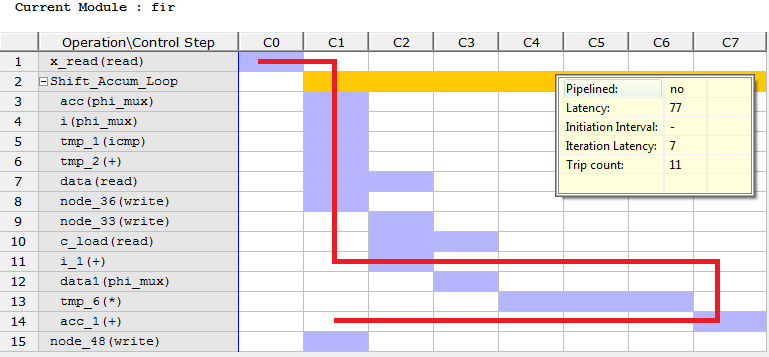
tab: Resources tab:
:

Performance
tab: Resources tab:
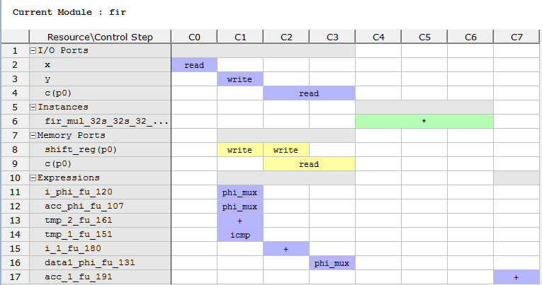
- x y . c , RAM;
- ;
- shift_reg ;
- , ( ).
:
The process of creating a new project and all the design steps will not be described, since the article has already grown to unprecedented size. But if you are interested in the topic of using Vivado HLS in my projects - I will be happy to share my experience. You can also use the help of habrauzer urock . In this case, he is a master!
Conclusion
On this I would like to summarize. The article describes the basic principles of creating FIR filters on FPGAs. General conclusions on the article:
- FIR filters are linear non-recursive filters that are fairly simple to implement on modern FPGAs and processors.
- Filter order = impulse response length = number of coefficients = number of delay lines.
- May have accurate linear phase response, constant group and phase delays.
- For linear phase response, symmetrical filter coefficients are required.
- Do not forget about the Gibbs effect when calculating the filter coefficients.
- When calculating the coefficients, use modern tools and do not reinvent the wheel.
- If the length of the filter N exceeds reasonable limits (for example, more than 512), use the fast convolution algorithm through double FFT.
- .
- .
- .
- , .
- . , .
Altera FIR Design:
Xilinx HLS FIR Design 1:
Xilinx HLS FIR Design 2:
Xilinx HLS FIR Design 1:
Xilinx HLS FIR Design 2:
- DSPLIB
- Altera FIR Compiler
- Xilinx FIR Compiler
- Xilinx DSP48E1 (7 Series)
- Xilinx DSP48E2 (Ultra-Scale)
- Wikipedia FIR
- Parks-McClellan algorithm
- MATLAB Tutorial 1
- MATLAB Tutorial 2
- OpenCores FIR 1
- OpenCores FIR 2
- OpenCores FIR 3
To be continued...
Source: https://habr.com/ru/post/274847/
All Articles