Create a hardware random number generator
I want to bring to your attention the hardware and software version of obtaining random numbers. Looking ahead, I will say that this option is not the only one, and this post opens up my small series of articles on getting, generating and studying random numbers, or, more precisely, just accidents.
')
The magic of random numbers attracted me from early childhood. Date of birth, death, giftedness, winning the lottery, exam ticket, etc. are all random events. On the other hand, looking at our world, you understand that there are no coincidences. Or, as scientists say: Accident is not a studied pattern. I was always wondering why this particular event is coming, and not another? Why is the coin, thrown now, fell headlong, and whether something can affect this event? What are the mutual influences of randomness on each other, can we influence these random variables? All these questions are still beyond science, but it is interesting to find the answer to them. Unfortunately, at the institute, I did not appreciate the subject “Theory of Probability” well enough and just passed it, for which I received a minus of life karma. By this, today I try my best to catch up.
For various engineering and computational problems requires the search for random numbers. Moreover, the higher the entropy of the number, the lower its regularity and predictability, the better. We all used in programming the function of the generator of random numbers. In fact, all these numbers are pseudo-random. They can be calculated using a very complex algorithm, or even be a “cast” of random system noise (such as / dev / random and / dev / urandom ). Yet, oddly enough, these random numbers are predictable. The most obvious way to get random numbers is to take them from the outside. After all, our real world is a huge random variable generator. Of course, all these quantities are also pseudo-random, but their patterns and interdependencies cannot be traced, due to the infinite number of variants of the events taking place. It should also be understood that one cannot consider random numbers as numbers appearing in a closed system, since they are influenced by an infinite number of external factors. Then, if you look, each event is completely non-random and has its own pattern. It is impossible to simply take into account all the mutual influences (and there are infinitely many); therefore, for simplicity, many events are taken as random.
The easiest way to get random numbers is to remove noise from a computer sound card. With that, the worse the sound card, the better it makes noise. As an additional source of noise, optionally, you can connect any radio tuned to noise to the line input of the sound card.
 +
+  + Sound card = Random generator
By the way, thermal noise in semiconductors, due to the thermal motion of atoms, is the most common source of random numbers, for example, when generating keys in SMART cards.
True, I want to note that there are known cases of hacking of devices with built-in encryption (SMART cards), which use the principle of thermal noise in semiconductors to generate random numbers. Hacking is quite simple - freezing in the liquid nitrogen of the chip itself, as a result of which the thermal noise drops to almost zero.
Random variables oscillate around a single value (the expectation of this value). We put, we remove a few thousand random points, find the maximum and minimum value, which takes a random variable. Take the interval from the minimum value that a random variable takes to the maximum value that a random variable can take. We divide this interval into equal intervals, for example, fifty. Ololo pysch-pysch, no one reads. And we calculate how many random variables fall into each interval, then we get a diagram of the distribution of a random variable. It must be said, the magnitude of the scattering of a random event is determined, and it is measured by dispersion. This method of constructing a scatterplot of a random variable is called interval. It is based on splitting the original numerical values into intervals.
If we imagine what a distribution is on our fingers, then it’s like we pour sand from a palm, in accordance with the change of the signal along the vertical axis.
I will illustrate with an example. Pendulum oscillations. If we expand it in time, we get a sinusoid f (x) = sin (x) - this is the original graph, the distribution of which we are looking for. If we add a salt shaker to this pendulum, which pours sand, then it will draw a distribution diagram. Let's demonstrate how it looks.
An example of a piece of code to build:
And the graph f (i) = a [i]

Graph of the "distribution" of the sine.
If we talk about the salt shaker on the pendulum, it becomes clear why such a schedule has turned out. At the highest point of the oscillation of the pendulum, which corresponds to the peaks of the sinusoid, the movement slows down and there the sand should form a "hill", and at the point of zero there should be a minimum amount of sand, because This place the pendulum passes with a maximum speed.
This is best demonstrated in this video, using the Galton board ru.wikipedia.org/wiki/Doska_Galtona , taken from the MEPhI lecture course
My institute also had a similar experience, and the teacher made a sacred phrase that made a big impression on me: I have been spending this experience for fifty years, and always get the same picture. Formally, nothing prevents particles from lying down evenly, but we always get a Gaussian distribution.
The Gauss distribution is subject to various quantities. For example, shooting at a target - bullets will fall in the target for the Gauss distribution. The most heap in the tens and least around the edges. Of course, electrical noise (if it is not caused by interference from the electrical network) will also obey this distribution.
There are other types of random variable distributions. For example, there is a Poisson distribution. One of the features of the Poisson distribution is that the random variable is discrete. The best illustration of the events of the Poisson distribution can be calls to any call-center. The number of calls received per unit of time will be a random variable. Or, while I was debugging a program, which I’ll talk about below, I measured the intervals for pressing a key. The intervals were measured by a microcontroller, counting the past number of cycles between each keystroke. I did a few thousand clicks and got just such a chart.
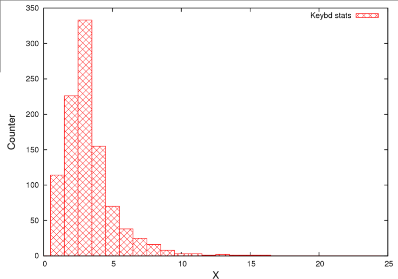
Chart of distribution of frequency of pressing the button.
By the way, I knowingly said that there are no random variables. Here I press a button with my finger. The randomness of the intervals of pressing is due to the fact that my brain is engaged in processing various signals, dreams of the "eternal", thoughts about the program, etc. Plus, the signals from the brain reach the limbs also not at the speed of light, because Ion exchange during signal transmission is caused by chemical processes in my body, etc. etc. As a result, we have a completely random intensity of clicks.
It should be noted that the registration of radioactive particles using dosimeters is also subject to the Poisson distribution.
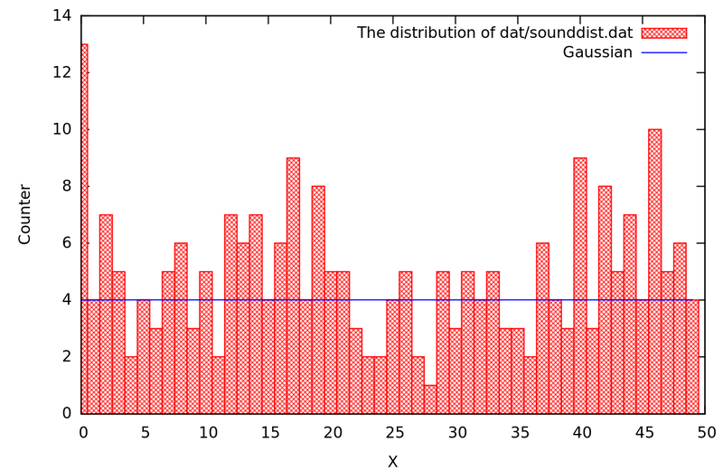
The most valuable distribution, from the programmer's point of view, is the uniform distribution. When random numbers are of any length, they are found equally often on the entire given range. An example from the life of such a distribution is the waiting time of transport at a bus stop, taking into account the fact that the transport runs at the same time intervals. You can come and immediately sit in a minibus, then your waiting time will be zero, or this minibus will go right from under your nose. Then your waiting time will be equal to the interval of minibuses. But, as a rule, you have to wait. And if we divide the waiting time into intervals dt and construct a histogram of the frequencies of hitting the minibus, say for several years, then it will be a line.

The histogram of the frequencies of hitting your bus.
Vertically, the number of hits on a minibus was postponed, and horizontally, the waiting time for a minibus.
For example, a histogram of the distribution of data received by / dev / random
Histogram of the system random number generator
You can get this histogram yourself by replacing / dev / audio (/ dev / dsp) with / dev / random in my program (which we will discuss below ) (initialization of the sound card does not affect the random number generator).
It should be noted that I have restarted the program 15 times in order to get the histogram closest to the theoretical one. This indicates the imperfection of this random number generator. The blue line shows how this histogram should look ideally.
Other types of distributions can be found in this figure.

The main types of distribution of random variables.
Taken from www.ievbras.ru/ecostat/Kiril/Library/Book1/Content350/Content351.htm .
Probably, I already managed to get bored with my amateur terver. By this, we move from theory to practice. My program is written under Linux, and tested on Ubuntu 10.10 . To build diagrams, the gnuplot package must be installed on the system; without it, the program will not work.
By the way, I strongly recommend that all engineers deal with the cross-platform software package gnuplot. This is the perfect package for building any graphs. After working with him, I forgot what plotting in MS Excel is like a bad dream. A day or two to figure out, and then at the laboratories at the institute or at work, you will delight yourself and others with original high-quality graphics. The undoubted plus that this package can be used in programs for quick and easy graphing.
I’ll not dwell on this story about gnuplot, how did I build graphs. It is better to write a separate post on this wonderful package.
So what does my program do? She within three seconds
With a sampling rate of 96,000 Hz
Writes data type signed short
From one sound card input channel
Data is saved to an array.
Then the sound card is initialized, and data is read for three seconds. I honestly admit that I didn’t explore all the features of working with a sound card. I did not try to read in stereo mode, to accept 24-bit data. I tried to change only the sampling rate. I also want to say that receiving data from a sound card is not always stable. After rebooting the system, I restart this program several times to get a histogram. Sometimes it produces completely incomprehensible values. With what it is connected, I also do not know.
After initializing the sound and reading all the data in the buf array, we find the minimum and maximum values of the array. After that, the non-sorted array is stored in array.dat (from which you can then build an oscillogram of the data to be removed). Next, the array is sorted by the function
For debugging, the sorted array is saved to the error.log file.
Next we find the delta - the interval of the cell in which we will add our values:
Allocate memory for the distribution array. Memory allocation is made for versatility so that you can dynamically change the size of the distribution.
After that, we start to consider what values fell into which interval, or in other words, build a distribution of random variables:
Already on this graph, you can build a diagram of the distribution of a random variable. But I want to compare the practical distribution with the theoretical schedule of the Normal distribution, which is based on the formula taken from Wikipedia ru.wikipedia.org/wiki/Normal_distribution :

To build on this formula, we need to find two parameters: Expectation and variance. As I said, mathematical expectation is a quantity around which random numbers fluctuate. Dispersion is a measure of dispersion. There are two ways to find these values - from the original array and from the resulting diagram. I find the mathematical expectation in two ways, but using the latter, I find the variance only in the last way.
The mathematical expectation in our case is simply the average of all random variables. We find it so
Variance is defined as the square deviation of a random variable from the expectation. We find it as follows:
Here:
gausse = (long double) summall * exp (- ((i-math_f) * (i-math_f)) / (2 * dispers)) / (sqrt (2 * 3.14159265 * dispers));
This is the calculation of the Gaussian distribution, using the expectation and variance.
The resulting program can be downloaded here: narod.ru/disk/32347266001/sound_distribution.tar.gz.html
After we compile the program with the make command.
For proper operation of the program you need to configure the sound card. In Ubunt, this is done like this: System-> Options- > Sound . Select the microphone input, set the volume to maximum and remove the checkbox “Turn off”. Optionally, you can connect a radio receiver to the line input of the sound card, then instead of the microphone input you can use the line input.
One note - the microphone must be disconnected from the sound card input. They say that throwing the microphone input is not worth it, so in principle it is possible to shunt (for those who wish) its resistance equal to the resistance of the microphone.
So, run the program "./sound_distribution" and admire the result after 3-4 seconds.
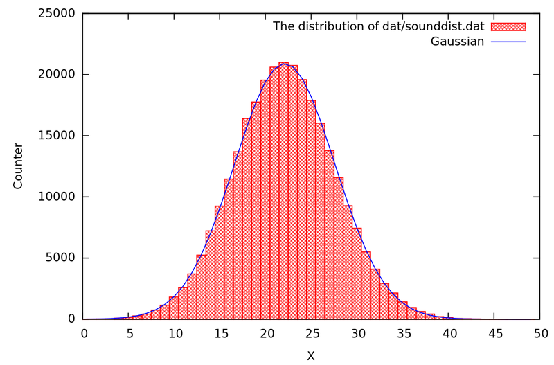
Histogram of the values obtained
Oscillogram of the obtained values from the microphone input.
The histogram turned out so successful that it can be inserted as an illustration in any textbook on the terver, although these are completely empirical values.
As I have already described, the programmer needs numbers that are evenly distributed. In this case, we have a normal distribution, where the number fluctuates around the expectation. To get the numbers we need, we must take the lower four bits of the number. These four bits will take a completely random value. And these four bits are laid in the number of the required length. For example, in order to fill a short number (2 bytes), we will need 4 numbers taken from the sound card, or rather their low-order bits. Here is a sample code:
Homework will be done so that the number can be generated in a given range and for different types of data. Well, so is the construction of the distribution for these random numbers :).
For the future, I wanted to make a program on GTK + so that the sliders can change the width of the intervals, the sampling rate, the amount of data received, the input data, etc. But alas, I have broken off my teeth for now. I made only the oscillogram graph of the received signal, riveting it from several programs. In this matter, I will be very grateful for all possible assistance.
Alternatively, you can put a stationary receiver, put a second sound card, purely for a random number generator. Write a daemon or driver that would have some sort of random data file, like / dev / random, from which data can be read. In general, the applications of mass.
I must say that the generation of random numbers in this way is relatively slow. It slows down the speed of reading data from a sound card. But in some, not critical to the speed of execution, tasks, it will be the most.
In fact, obtaining random numbers from a sound card was a by-product of my personal little research, and in this case, serves me only for running in of my modest algorithms and data visualization.
My program saves three files:
array.dat - This is just the raw data of the captured array.
error.log - this file was supposed (as the name implies) to save errors, but for the time being it is used to save an ordered array. Which, in general, served me for debugging.
sounddist.dat - The output file itself. In the first column, the ordinal number of the column of the diagram, the second column is the value of the relative frequencies, the third is the Gaussian distribution calculated by the standard formula, the fourth is the range of values that fall into this column of the diagram.
I don't know why, but #define stopped working in this program. Attempting to initialize a variable using define results in an error. For example, if you replace: “arg = 16;” (line 83) with “arg = SIZE;” (comment out line 83 and uncomment line 79), the compiler will generate an error:
sound_distribution.c: In function 'main':
sound_distribution.c: 81: error: stray '\ 321' in program
sound_distribution.c: 81: error: stray '\ 216' in program
make: *** [sound_distribution] Error 1
The funny thing is that in the original program, the initialization of variables goes through defines. The lack of defaults makes the code not very convenient for editing, but a brief googling did not give an answer to this problem.
Error found and fixed, thanks galaxy
As a conclusion, I want to say that the hardware random number generator is very easy to get; you just have to look around :).
I will appreciate any constructive criticism, ranging from the style of writing programs, ending with algorithms. I would also be grateful for any feasible assistance in the continuation of the project on GTK +.
I also want to say that this post is not the last on this topic.
1. ru.wikipedia.org/wiki/Normal_distribution
2. en.wikipedia.org/wiki/ Distribution_ Poisson
3. tegir.ru/ml/k66.html hardware random number generator.
4. www.mtu-net.ru/aborovsky/articles/linsnd1.htm Sound Programming in Linux (rus)
5. www.oreilly.de/catalog/multilinux/excerpt/ch14-05.htm example of the Linux audio program that is used in my program.
Added:
6. N.S. Markin "Fundamentals of the theory of processing measurement results"
7. habrahabr.ru/blogs/python/62237 Random numbers from a sound card
The bibliography will still be supplemented and expanded, because now I don’t have all those books that I used when writing the program, understanding the server and writing this post.
')
The magic of random numbers attracted me from early childhood. Date of birth, death, giftedness, winning the lottery, exam ticket, etc. are all random events. On the other hand, looking at our world, you understand that there are no coincidences. Or, as scientists say: Accident is not a studied pattern. I was always wondering why this particular event is coming, and not another? Why is the coin, thrown now, fell headlong, and whether something can affect this event? What are the mutual influences of randomness on each other, can we influence these random variables? All these questions are still beyond science, but it is interesting to find the answer to them. Unfortunately, at the institute, I did not appreciate the subject “Theory of Probability” well enough and just passed it, for which I received a minus of life karma. By this, today I try my best to catch up.
Formulation of the problem
For various engineering and computational problems requires the search for random numbers. Moreover, the higher the entropy of the number, the lower its regularity and predictability, the better. We all used in programming the function of the generator of random numbers. In fact, all these numbers are pseudo-random. They can be calculated using a very complex algorithm, or even be a “cast” of random system noise (such as / dev / random and / dev / urandom ). Yet, oddly enough, these random numbers are predictable. The most obvious way to get random numbers is to take them from the outside. After all, our real world is a huge random variable generator. Of course, all these quantities are also pseudo-random, but their patterns and interdependencies cannot be traced, due to the infinite number of variants of the events taking place. It should also be understood that one cannot consider random numbers as numbers appearing in a closed system, since they are influenced by an infinite number of external factors. Then, if you look, each event is completely non-random and has its own pattern. It is impossible to simply take into account all the mutual influences (and there are infinitely many); therefore, for simplicity, many events are taken as random.
The easiest way to get random numbers is to remove noise from a computer sound card. With that, the worse the sound card, the better it makes noise. As an additional source of noise, optionally, you can connect any radio tuned to noise to the line input of the sound card.
+ + Sound card = Random generatorBy the way, thermal noise in semiconductors, due to the thermal motion of atoms, is the most common source of random numbers, for example, when generating keys in SMART cards.
True, I want to note that there are known cases of hacking of devices with built-in encryption (SMART cards), which use the principle of thermal noise in semiconductors to generate random numbers. Hacking is quite simple - freezing in the liquid nitrogen of the chip itself, as a result of which the thermal noise drops to almost zero.
The histogram of the frequency of the number of observations of a random variable
Random variables oscillate around a single value (the expectation of this value). We put, we remove a few thousand random points, find the maximum and minimum value, which takes a random variable. Take the interval from the minimum value that a random variable takes to the maximum value that a random variable can take. We divide this interval into equal intervals, for example, fifty. Ololo pysch-pysch, no one reads. And we calculate how many random variables fall into each interval, then we get a diagram of the distribution of a random variable. It must be said, the magnitude of the scattering of a random event is determined, and it is measured by dispersion. This method of constructing a scatterplot of a random variable is called interval. It is based on splitting the original numerical values into intervals.
If we imagine what a distribution is on our fingers, then it’s like we pour sand from a palm, in accordance with the change of the signal along the vertical axis.
I will illustrate with an example. Pendulum oscillations. If we expand it in time, we get a sinusoid f (x) = sin (x) - this is the original graph, the distribution of which we are looking for. If we add a salt shaker to this pendulum, which pours sand, then it will draw a distribution diagram. Let's demonstrate how it looks.
An example of a piece of code to build:
do { y=512*sin(x)+512; count=0; for (i=0;i<n;i++) { if ( y<count+deltay && y >=count) { a[i]=a[i]+1; break; } count=count+deltay; } x=x+deltax; } while (x<200*3.14159265); And the graph f (i) = a [i]
Graph of the "distribution" of the sine.
If we talk about the salt shaker on the pendulum, it becomes clear why such a schedule has turned out. At the highest point of the oscillation of the pendulum, which corresponds to the peaks of the sinusoid, the movement slows down and there the sand should form a "hill", and at the point of zero there should be a minimum amount of sand, because This place the pendulum passes with a maximum speed.
Gaussian distribution or normal
This is best demonstrated in this video, using the Galton board ru.wikipedia.org/wiki/Doska_Galtona , taken from the MEPhI lecture course
My institute also had a similar experience, and the teacher made a sacred phrase that made a big impression on me: I have been spending this experience for fifty years, and always get the same picture. Formally, nothing prevents particles from lying down evenly, but we always get a Gaussian distribution.
The Gauss distribution is subject to various quantities. For example, shooting at a target - bullets will fall in the target for the Gauss distribution. The most heap in the tens and least around the edges. Of course, electrical noise (if it is not caused by interference from the electrical network) will also obey this distribution.
Poisson distribution
There are other types of random variable distributions. For example, there is a Poisson distribution. One of the features of the Poisson distribution is that the random variable is discrete. The best illustration of the events of the Poisson distribution can be calls to any call-center. The number of calls received per unit of time will be a random variable. Or, while I was debugging a program, which I’ll talk about below, I measured the intervals for pressing a key. The intervals were measured by a microcontroller, counting the past number of cycles between each keystroke. I did a few thousand clicks and got just such a chart.
Chart of distribution of frequency of pressing the button.
By the way, I knowingly said that there are no random variables. Here I press a button with my finger. The randomness of the intervals of pressing is due to the fact that my brain is engaged in processing various signals, dreams of the "eternal", thoughts about the program, etc. Plus, the signals from the brain reach the limbs also not at the speed of light, because Ion exchange during signal transmission is caused by chemical processes in my body, etc. etc. As a result, we have a completely random intensity of clicks.
It should be noted that the registration of radioactive particles using dosimeters is also subject to the Poisson distribution.
Uniform distribution
The most valuable distribution, from the programmer's point of view, is the uniform distribution. When random numbers are of any length, they are found equally often on the entire given range. An example from the life of such a distribution is the waiting time of transport at a bus stop, taking into account the fact that the transport runs at the same time intervals. You can come and immediately sit in a minibus, then your waiting time will be zero, or this minibus will go right from under your nose. Then your waiting time will be equal to the interval of minibuses. But, as a rule, you have to wait. And if we divide the waiting time into intervals dt and construct a histogram of the frequencies of hitting the minibus, say for several years, then it will be a line.
The histogram of the frequencies of hitting your bus.
Vertically, the number of hits on a minibus was postponed, and horizontally, the waiting time for a minibus.
For example, a histogram of the distribution of data received by / dev / random
Histogram of the system random number generator
You can get this histogram yourself by replacing / dev / audio (/ dev / dsp) with / dev / random in my program (which we will discuss below ) (initialization of the sound card does not affect the random number generator).
It should be noted that I have restarted the program 15 times in order to get the histogram closest to the theoretical one. This indicates the imperfection of this random number generator. The blue line shows how this histogram should look ideally.
Other types of distributions can be found in this figure.
The main types of distribution of random variables.
Taken from www.ievbras.ru/ecostat/Kiril/Library/Book1/Content350/Content351.htm .
Less words and more deeds
Probably, I already managed to get bored with my amateur terver. By this, we move from theory to practice. My program is written under Linux, and tested on Ubuntu 10.10 . To build diagrams, the gnuplot package must be installed on the system; without it, the program will not work.
By the way, I strongly recommend that all engineers deal with the cross-platform software package gnuplot. This is the perfect package for building any graphs. After working with him, I forgot what plotting in MS Excel is like a bad dream. A day or two to figure out, and then at the laboratories at the institute or at work, you will delight yourself and others with original high-quality graphics. The undoubted plus that this package can be used in programs for quick and easy graphing.
I’ll not dwell on this story about gnuplot, how did I build graphs. It is better to write a separate post on this wonderful package.
So what does my program do? She within three seconds
#define LENGTH 3 /* how many seconds of speech to store */ With a sampling rate of 96,000 Hz
#define RATE 96000 /* the sampling rate */ Writes data type signed short
#define SIZE 16 /* sample size: 8 or 16 bits */ From one sound card input channel
#define CHANNELS 1 /* 1 = mono 2 = stereo */ Data is saved to an array.
short buf[LENGTH*RATE*SIZE*CHANNELS/16]; Then the sound card is initialized, and data is read for three seconds. I honestly admit that I didn’t explore all the features of working with a sound card. I did not try to read in stereo mode, to accept 24-bit data. I tried to change only the sampling rate. I also want to say that receiving data from a sound card is not always stable. After rebooting the system, I restart this program several times to get a histogram. Sometimes it produces completely incomprehensible values. With what it is connected, I also do not know.
After initializing the sound and reading all the data in the buf array, we find the minimum and maximum values of the array. After that, the non-sorted array is stored in array.dat (from which you can then build an oscillogram of the data to be removed). Next, the array is sorted by the function
quickSortR(buf, lbuf); For debugging, the sorted array is saved to the error.log file.
Next we find the delta - the interval of the cell in which we will add our values:
deltay=(unsigned short)((max-min)/n_rasp+1); Allocate memory for the distribution array. Memory allocation is made for versatility so that you can dynamically change the size of the distribution.
rasp = (unsigned int *)(malloc(n_rasp*sizeof(unsigned int))); After that, we start to consider what values fell into which interval, or in other words, build a distribution of random variables:
for (i=0;i<n;i++) { count=min; for (j=0;j<n_rasp;j++) { if ((buf[i] >=count) && (buf[i]<=count+deltay)) { rasp[j]++; break; } count=count+deltay; } } Already on this graph, you can build a diagram of the distribution of a random variable. But I want to compare the practical distribution with the theoretical schedule of the Normal distribution, which is based on the formula taken from Wikipedia ru.wikipedia.org/wiki/Normal_distribution :
To build on this formula, we need to find two parameters: Expectation and variance. As I said, mathematical expectation is a quantity around which random numbers fluctuate. Dispersion is a measure of dispersion. There are two ways to find these values - from the original array and from the resulting diagram. I find the mathematical expectation in two ways, but using the latter, I find the variance only in the last way.
The mathematical expectation in our case is simply the average of all random variables. We find it so
for (i=0;i<n_rasp;i++) { summall=rasp[i]+summall; math_f+=rasp[i]*i; } printf("math_f = %3.5f sumall=%d\n",math_f,summall); math_f=math_f/summall; printf(" 2 = %3.5f\n",math_f); Variance is defined as the square deviation of a random variable from the expectation. We find it as follows:
for (i=0;i<n_rasp;i++) { dispers+=((long double)(i)-math_f)*((long double)(i)-math_f)*(rasp[i]); } dispers=dispers/summall; printf(" = %4.5Lf\n",dispers); ... // for (i=0;i<n_rasp;i++) { gausse=(long double)summall*exp(-((i-math_f)*(i-math_f))/(2*dispers))/(sqrt(2*3.14159265*dispers)); fprintf(logf, "%3ld %5d %+07.5Lf (%10d;%10d]\n",i,rasp[i], gausse ,dat, dat+deltay); //write to file } .... // : gnuplot(outputfile, 0, 0); gnuplot("dat/array.dat", 1, 0); Here:
gausse = (long double) summall * exp (- ((i-math_f) * (i-math_f)) / (2 * dispers)) / (sqrt (2 * 3.14159265 * dispers));
This is the calculation of the Gaussian distribution, using the expectation and variance.
The resulting program can be downloaded here: narod.ru/disk/32347266001/sound_distribution.tar.gz.html
After we compile the program with the make command.
For proper operation of the program you need to configure the sound card. In Ubunt, this is done like this: System-> Options- > Sound . Select the microphone input, set the volume to maximum and remove the checkbox “Turn off”. Optionally, you can connect a radio receiver to the line input of the sound card, then instead of the microphone input you can use the line input.
One note - the microphone must be disconnected from the sound card input. They say that throwing the microphone input is not worth it, so in principle it is possible to shunt (for those who wish) its resistance equal to the resistance of the microphone.
So, run the program "./sound_distribution" and admire the result after 3-4 seconds.
Histogram of the values obtained
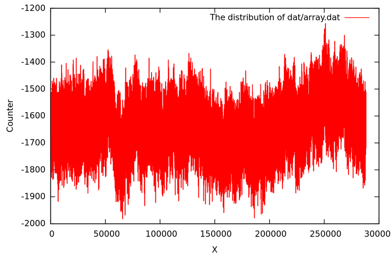
Oscillogram of the obtained values from the microphone input.
The histogram turned out so successful that it can be inserted as an illustration in any textbook on the terver, although these are completely empirical values.
Practical application
As I have already described, the programmer needs numbers that are evenly distributed. In this case, we have a normal distribution, where the number fluctuates around the expectation. To get the numbers we need, we must take the lower four bits of the number. These four bits will take a completely random value. And these four bits are laid in the number of the required length. For example, in order to fill a short number (2 bytes), we will need 4 numbers taken from the sound card, or rather their low-order bits. Here is a sample code:
short random_num=0; for (i=n; i<n+4; i++) { random_num<<= 4; random_num+=buf[i]&0x0F; } Homework will be done so that the number can be generated in a given range and for different types of data. Well, so is the construction of the distribution for these random numbers :).
Future plans
For the future, I wanted to make a program on GTK + so that the sliders can change the width of the intervals, the sampling rate, the amount of data received, the input data, etc. But alas, I have broken off my teeth for now. I made only the oscillogram graph of the received signal, riveting it from several programs. In this matter, I will be very grateful for all possible assistance.
Alternatively, you can put a stationary receiver, put a second sound card, purely for a random number generator. Write a daemon or driver that would have some sort of random data file, like / dev / random, from which data can be read. In general, the applications of mass.
Notes and conclusions
I must say that the generation of random numbers in this way is relatively slow. It slows down the speed of reading data from a sound card. But in some, not critical to the speed of execution, tasks, it will be the most.
In fact, obtaining random numbers from a sound card was a by-product of my personal little research, and in this case, serves me only for running in of my modest algorithms and data visualization.
My program saves three files:
array.dat - This is just the raw data of the captured array.
error.log - this file was supposed (as the name implies) to save errors, but for the time being it is used to save an ordered array. Which, in general, served me for debugging.
sounddist.dat - The output file itself. In the first column, the ordinal number of the column of the diagram, the second column is the value of the relative frequencies, the third is the Gaussian distribution calculated by the standard formula, the fourth is the range of values that fall into this column of the diagram.
Error found and fixed, thanks galaxy
As a conclusion, I want to say that the hardware random number generator is very easy to get; you just have to look around :).
I will appreciate any constructive criticism, ranging from the style of writing programs, ending with algorithms. I would also be grateful for any feasible assistance in the continuation of the project on GTK +.
I also want to say that this post is not the last on this topic.
Bibliography
1. ru.wikipedia.org/wiki/Normal_distribution
2. en.wikipedia.org/wiki/ Distribution_ Poisson
3. tegir.ru/ml/k66.html hardware random number generator.
4. www.mtu-net.ru/aborovsky/articles/linsnd1.htm Sound Programming in Linux (rus)
5. www.oreilly.de/catalog/multilinux/excerpt/ch14-05.htm example of the Linux audio program that is used in my program.
Added:
6. N.S. Markin "Fundamentals of the theory of processing measurement results"
7. habrahabr.ru/blogs/python/62237 Random numbers from a sound card
The bibliography will still be supplemented and expanded, because now I don’t have all those books that I used when writing the program, understanding the server and writing this post.
Source: https://habr.com/ru/post/274833/
All Articles