How to predict a stock price: An adaptive filtering algorithm

A group of Brazilian scientists has published a study on the creation of a tool for predicting the behavior of assets traded on the stock market. The paper presents a detailed description of the method and method of calculation for such forecasts. We present to your attention the most interesting moments of this document.

What is an adaptive filter

An adaptive filter is a tool that is capable of learning to achieve a given level of correspondence of the output to the real state of affairs. By adaptability is meant the ability to respond to changes in input data in real time to achieve higher performance. In practice, adaptive algorithms are implemented by two classical methods - the gradient method and least squares (LMS and RLS). Such a filter can be used for a wide range of tasks - filtering, spectral analysis or search for signals, etc.
')
Figure 1 shows the universal scheme for applying an adaptive filter in a predictive framework, where k is the iteration number, x (k) is the incoming signal, y (k) is the output of the adaptive filter, which is the prediction of the desired answer d (k), and e (k ) - error signal, defined as the difference between the desired response and the output of the filter, that is, e (k) = d (k) - y (k).

The recursive adaptive least squares algorithm (RLS, recursive Least-Squares) makes it possible to achieve high performance and speed of convergence when used in time-varying media.



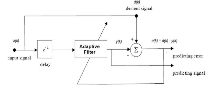
Fig. 1. General block diagram of an adaptive filter for signal prediction

Another important parameter is the so-called observation window, that is, the time period of the analysis, which usually has a rectangular or exponential correspondence. The parameter controlling the correspondence and duration of the observation window is called forgetting coefficients λ (it is applied to the algorithm's memory), 0 << λ < 1 and the object function looks like this: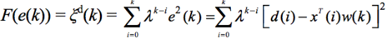



This function is convex in the multidimensional space w(k) , that is, ξ ^d (k) has only one global minimum and no local minimum. Thus, we can reach this point by setting the gradient ξ ^d (k) to zero, which will lead to the following formula: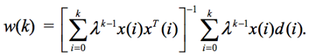

Using an adaptive filter in the stock price prediction framework

The purpose of this study is to understand how viable is the option of using adaptive filtering as a tool for predicting stock prices on real exchanges. An adaptive LMS filter was successfully used to predict traffic in wireless networks [Liang (2002)]. In the current case, adaptive filtering was used to obtain an estimate of the possible value of the shares of Petrobras shares traded on the Brazilian Bovespa Stock Exchange in São Paulo (ticker PETR3).

In order to create a PETR3 price movement prediction module, an adaptive digital FIR filter with 100 real coefficients was used. RLS with a forgetting factor of 0.98 was used as an adaptation algorithm. A predictability window of 16 days was also used. The simulation was performed on the MATLAB platform, trade information was used as input data from 01/03/2000 to 09/23/2009. The values ​​of the daily stock prices correspond to the closing time of the auction. Figure 2 shows the convergence of the coefficients of the adaptive filter used in the creation of the PETR3 price movement predictions.



Fig. 2. Convergence of the coefficients of an adaptive filter launched to generate Petrobras stock price predictions (PETR3 on the Brazilian stock market).

The evolution of the filter coefficients clearly demonstrates the presence of convergence in a period that approximately coincides with the prediction time. The abscissa shows the number of trading days involved in the simulation. The real valuation of PETR3 stocks on the Brazilian stock market during this period is shown by the red line in Figure 3. There, the black prices for the filter are also indicated.



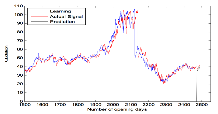
Fig. 3. PETR3 share price in the Brazilian stock market during the analysis period for filtering. Red shows the real market trend, black shows the estimate generated by the adaptive filter.

Obviously, there is a correspondence between the predicted prices and how things were actually in the market. To confirm this fact, a specific trading day was simulated - specifically, 2,450 days from the beginning of the observations of 1/3/2000 year. Figure 4 shows the zoom of the prediction made by the adaptive filter:



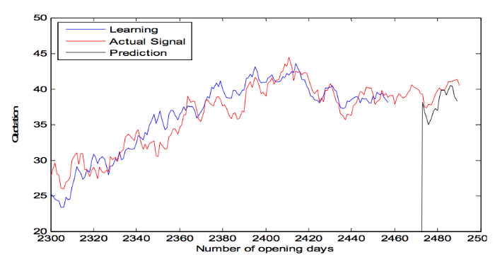
Fig. 4. Prediction of stock prices on a specific day

Adaptive filter performance for predicting selected asset prices

Consider the strategy of investing in PETR3 stocks using predictions generated by the filter since 2473 (shown in Figure 5). Filtering is performed using an RLS-algorithm with 100 coefficients and a forgetting coefficient λ = 0.98. The estimated trend of PETR3 stock price movements for the 16-day window is shown by a dotted line in Figure 5.



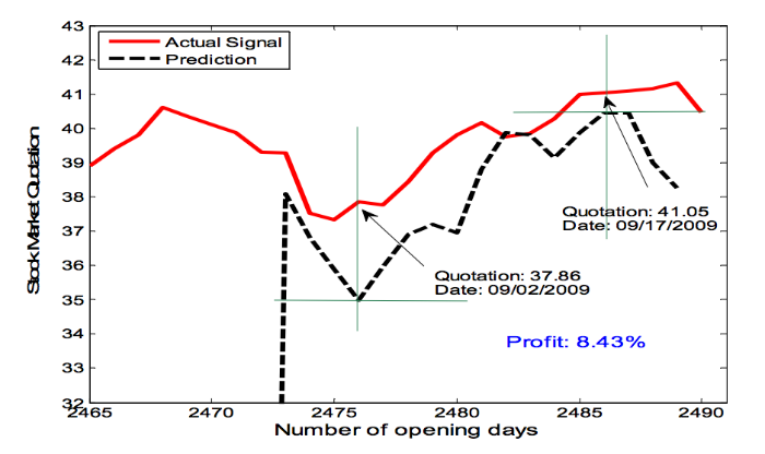
Fig. 5. The behavior of the asset PETR3 in the period from 08/18/2009 to 09/22/2009. Dotted line - prediction of the adaptive filter, red - the real price of shares on the market.

The prediction curve indicates the need to purchase an asset on the trading day of 09/02/2009 and the sale of shares at the time of 09/17/2009 - thus the sale should occur at the time of the rise preceding the price reduction. The real price chart suggests that if such a strategy were implemented, the purchase of shares would pass at a price of 37.86, and the sale would be at 41.05, which would yield a profit of 8.43% of the volume of investments. Although this example is only a special case, it illustrates the possible effectiveness of predictions based on adaptive filtering. Further tests were conducted for other trading days, and the results were generally the same.

Creating an adaptive filter and prediction accuracy

Despite the positive test results, the proposed method leaves some questions. One of them sounds like this - for which type of assets does it work better? How many FIR coefficients should be used to improve the quality of the prediction module? Does the result affect the value of the forgetting coefficient?

To assess the quality of predictions made using adaptive filtering, a correlation is used - this is a measure of similarity for analyzing the quality of the match between the predicted signal and real quotes on the stock exchange within a given prediction window.

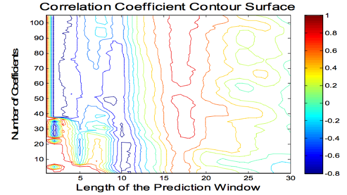
The accuracy analysis is performed by studying the correlation values ​​as a function of the number of filter coefficients and the size of the prediction window. Figure 5 shows a 3D graph of the correlation between 08/18/2009 and 09/22/2009:



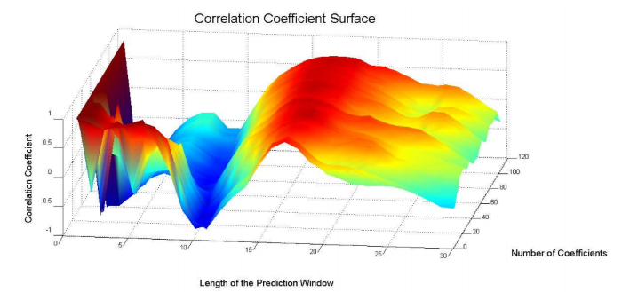
Fig. 6. Correlation 3D-graph between the predicted signals and real stock quotes.

Chart 6 was converted to a three-dimensional contour chart presented in Figure 7. It shows better the zone of increased correlation between the generated predicted signal and the real stock prices in the market.



To study the effect of the number of filter coefficients for adaptive predictions, a side space profile was created from Figure 6 (shown in Fig. 8), which shows correlation peaks visible to an observer located in the right side of the space. Obviously, the region between the 30 and 100 coefficients represents a high correlation. Accordingly, using 30 or fewer coefficients is not enough to get an accurate prediction.



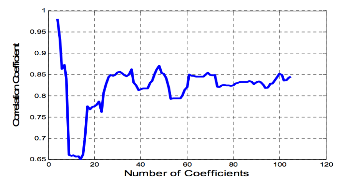
Fig. 8. Correlation profile, taking into account the number of coefficients.

The first section of high correlation is not particularly useful, since it can only be achieved with a very small prediction window. The best option in this particular scenario is to choose the number of coefficients between 60 and 100.

Then, in order to assess the influence of the prediction window on the quality of the predictions obtained, the front profile of the three-dimensional space from Figure 6 was created (Fig. 9). It shows the behavior of the maximum correlation based on the size of the prediction window. Obviously, the choice of a very short window leads to a high correlation (indeed, the prices of stocks of trading days following one another show a high correlation). However, this gives us practically nothing in terms of creating investment strategies in the stock market.



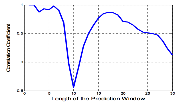
Fig. 9. Correlation profile taking into account the size of the prediction window (from 1 to 30 trading days of the Brazilian stock market).

An unexpected result - experiments showed that the choice of a prediction window measuring about 10 days is extremely inefficient. In contrast, predictions on the window in about 15 business days show much better results. Just as it was supposed, too long prediction windows lead to a decrease in correlation.

Thus, the most optimal prediction window in this particular case is 15-20 days.

Table 1 presents a summary of the number of coefficients used, the length of the prediction window, the date of purchase and sale of shares according to the proposed strategy of the filter, the price of transactions, as well as the total profit of transactions.



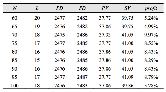
As can be seen, the use of an adaptive filter made it possible to achieve a profit, on average, in the amount of 7% of the volume of investments.