Using Matalysis in computer games (part 2)
Keywords: collection task; Wolfram Alpha; Wolfram Mathematica; Stirling numbers of the second kind; mathematical analysis; probability theory; mat waiting; median; quantile; computer games; liner collection; distribution function of a random variable; probability density, ArcheAge.
When it remains to get only three of the hundred items in order to collect the entire collection (inserts of BomBimBomb gum or Turbo, or a set of heavy armor for a computer game character), then the fire in the eyes and waiting for a miracle suppress both logic and intelligence and mathematical analysis from the head completely . There is only one thought “A little bit more and I’ll get the rest! I will collect all! At this time, relatives and friends of this obsessed collector are puzzled with only one question - “Oh, a little bit, how much ?!”. How many mothers need to buy more hateful chewing gums, or how many more girls need to sit alone, until her boyfriend knocks out the “most rare pants of Baal” from monsters ?!
Answering the question “how much to buy chewing gum to assemble a complete collection of N-pieces of inserts” is quite difficult at once, even if you use Yandex, because it is difficult to formulate the query itself for an “ordinary” search engine. Attempting to solve the problem yourself usually puts people at a dead end - it’s not clear which way to approach it.
This article will address three questions: How to approach tasks that are not clear at first glance how to solve? What search engine to use in order to receive scientific answers to scientific questions (and not to receive offers to buy a quadratic equation on eBay)? And of course, how much does one need to buy chewing gum to assemble a collection of liners?
The article was quite large. Therefore, in those places where you can miss something, I will report about it. In such chapters will be considered not the solution of the problem, but those concepts and principles that are used when solving it. If the details become interesting, you can re-read the missing places later. The wording of the task should be reviewed, but further, those who want to get acquainted with the answer as soon as possible can go directly to the results. I advise, however, separately to familiarize with the chapter devoted to Alpha Wolfram .
Also for convenience, I cite a complete list of chapters.
')
To make it clear to those who love mathematical rigor, and to those who are not familiar with it, I will formulate the collection problem in two ways.
We will immediately clarify a number of points that will further help us in the decision. First, for simplicity, all elements of the collection will be numbered from 1 to K, and thus simply deal with numbers. Secondly, our elementary outcomes will be sequences of numbers of length N, consisting of K different numbers. For example, if K = 3 and N = 5, then the sequences {3,3,1,2,3}, {1,2,3,3,3}, {3,3,1,1,1} are one of possible outcomes, and the order of the elements matters. If in such a sequence all K numbers occur, at least once - this means a “successful” sequence for us, if it does not occur, at least one number never, then the sequence is not successful for us. Moreover, any possible sequence is equally probable. Thirdly, we can always count the number of all possible sequences of K numbers, the length of N elements, provided that the order matters. This number is K ^ N. Fourth, the probability of collecting a collection in N steps is equal to the ratio of "successful" sequences to the total, that is, to K ^ N. Thus, it is possible to search for either the probability or the number of “successful” sequences - as it will be more convenient, one can always be obtained from the other.
Those who have no questions about "order matters" and "quantity is K ^ N", as well as who remembers what "factorial" and "C from n to k" are, you can skip this chapter and go on to the next one . For those who have thoroughly forgotten combinatorics, or have not yet been acquainted with it, consider the main points that will be useful to us.
The history of combinatorics, though rooted in deep antiquity, still actively developed thanks to gammers. Well, maybe Cardano, Galileo, Farm Pascal and the rest of the great minds of the world themselves were not avid gamers (though not a fact, not a fact), but at least their gamers specifically bothered with questions about games, about winning strategies, asked for guides to write. Of course, then more than dice and cards were played, gambling fans with tanks or magic were somehow not very many. With one there was a shortage, and for the other burned. But actively applied to the analysis of puzzles and gambling, combinatorics was extremely useful for solving practical problems in almost all branches of mathematics. In addition, combinatorial methods have proven useful in statistics, programming, genetics, linguistics, and many other sciences a long time later. Wikipedia EVIL (I’ll remember this more than once), but reviewing things not related to formulas is physically possible to read there, but you shouldn’t trust them. Nevertheless, you can read the article "History of combinatorics"
While I was looking for various materials on combinatorics, I came across a site , or rather, one of the documents from this site. I liked the language with which it is written, you can get acquainted with the combinatorics there. I, in general, would not have remembered this site, if not for one “but”. There is a problem about the trajectory. I liked it very much, it seemed interesting, and looking at it, I had an idea how to solve the problem about the collection, but more on that later.
Here are the basic facts from combinatorics, which will be useful to us.
1.) What is the total number of N -digit numbers in the number system with base K? In how many ways can representatives of K nations be placed on the N chairs? How many ways can you color N squares if there are markers of K different colors? In how many ways can you fill N boxes with multi-colored balls, if the number of different colors K and only one ball fit into each box?
The answer to all these questions is one - “Accommodation with repetitions”. In the case of balls, in the first box we can put a ball of any of K colors. That is, we have K options to shove one ball in the first box. In the second box we can also shove the ball in K ways. The options for filling the first and second boxes with balls will already be K * K = K ^ 2. This happens because for each option of filling the first box there can be any of K options for filling the second box. If we have N boxes, then the options will be K ^ N.
2.) How many there are N -digit numbers in the number system with the base N, such that each digit in the number occurs exactly once? In how many ways can representatives of N nations be placed on the N seats, so that a representative of each nation sits? How many ways can you color N squares, if there are markers of N different colors, so that each marker can be used (without repainting, of course)? How many ways can you fill N boxes with N numbered balls?
The answer to all these questions is one - "Rearrangement". Cases with balls and numbers, in general, are identical, even in their wording. In the first place we can put any of the N balls. On the second place is any of the remaining N-1 balls, on the third one of the remaining N-2 balls after filling the first two places. And so on until the last. It turns out that we have the product N * (N-1) * (N-2) * (N-3) * ... * (N- (N-2)) * (N- (N-1)). Here is the product of all natural numbers from 1 to N and is called factorial. And it is designated as “N!”. Yes, an exclamation mark, this is the designation of factorial or product of all natural numbers from 1 to N. It is extremely common everywhere, and considering that writing it in the form of a work for quite a long time, we decided to simplify and shorten the record to the exclamation mark icon. There is an old joke about factorial that teachers love to tell.
At the matane exam, the lecturer asks the student to expand the exhibitor into a Taylor series.
Student: One plus X divided into ONE (pronounces loudly and solemnly) plus X in the square divided into TWO (also loudly) plus X in the cube divided into THREE
Lecturer: Okay, okay, it's all right, just why are you screaming like that ?!
Student: Well, the exclamation point is the same !!!
It should be noted that the factorial from zero is 1. 0! = 1
3.) In how many ways can K boxes be filled with numbered balls? (balls more than boxes) You have N movie tickets and K girlfriends. How many ways can you hand out tickets to your friends? (there are more tickets than friends)
The answer to these questions is “Accommodation WITHOUT repetition”. However, the decision is similar not to the first point, but to the second. In the first place we can put any of the N balls. On the second place is any of the remaining N-1 balls, on the third one of the remaining N-2 balls after filling the first two places. And so on until the drawers run out. So, the product will be N * (N-1) * (N-2) * (N-3) * ... * (N- (K-1)). That is, the product of all natural numbers from K + 1 to N. But such a product can be painted as N * (N-1) * (N-2) * (N-3) * ... * (N- (K-1)) * (NK)! / (NK)! = N! / (NK)! That, in general, is significantly shorter.
4.) The last point is about why order may or may not matter. And what is "C from n to k".
Suppose you have a UAZ, and you are going to go with friends (only guys, without girls) for fishing. In the UAZ can climb K people. And all in all you have N. friends. Anyone who does not fit into your UAZ will drive other cars. How many options are there to fill in your friends with UAZ? How many ways are there of 20 (N) of your friends who are now online to assemble a team of 5 people (K) in order to play dota for an hour? (Of course there is a nuance - to consider you or not, but we will not bother with it)
What is the difference of this example from all previous ones? That order does not matter. Who, how and where will sit in the UAZ, or who you are first, and who will call the second to the team, no matter what role. The main thing is the composition, and who is where it is no longer important. If order were important, it would be exactly the previous version, that is, the answer would be N! / (NK) !. But order is not important to us. And about the order we had an example 2) with factorial. That is, N! / (NK)! must be divided into K !, and then the cases, which differed only in sequence, but were identical in composition, “would collapse into one variant.” For example, let there be 3 people and 2 places. Then all the possible options. For example 3 will be {1,2}, {1,3}, {2,1}, {2,3}, {3,1}, {3,2}. That is, 6 options. 3! / (3-2)! = 3! / 1! = 3! = 6. But in our example with a UAZ (the double truth is now UAZ), the sequence is not important and therefore the options like {1,2} and {2,1} are the same. Well, really, Petya and Vasya in UAZ or Vasya and Petya - there is no difference. The main thing that they two go in it. We get that the answer for point 4, in which order does not matter, is the formula N! / (NK)! / K! And there are such cases when the order is not important, and only the composition is “Combined from N to K”. There is another name for this miracle formula - “Binomial coefficient”. But most often it is called “C of n by k”. ("Tse from en ka"). It is denoted by the letter C with the subscript and the superscript n and k, respectively. The binomial coefficient is directly related to the well-known "Newton binomic." There is nothing difficult in it, you can read about it where you want (Just do not read the main Wikipedia). Newton's binomial and binomial coefficients are inherently quite simple, but the fact that they suddenly suddenly turn out to be applicable in an incredibly large number of different situations creates a sort of mystical aura and the suspicion that this is all for a reason. Although there is nothing complicated there, but a lot of interesting things.
This knowledge of combinatorics at this stage will be enough, the rest will be explained along the way.
When I first tried to solve the problem analytically, trying to honestly count (not by enumeration of course, but with formulas) all possible sequences satisfying the conditions, I confess nothing happened. More precisely, the path of reasoning was quite logical, but in the end I came to the need to write a huge amount of sums, which could not be rolled up into something compact.
In cases when the basic principles of some process are clear, but we cannot get a sensible and digestible law describing this process (when we understand what is happening and how, but the formula for this whole business does not work out), then you can go from the opposite - simulate this process, get a numerical solution and try to analyze the answer. For example, using the greatest of the methods of analysis is the “Close Look Method”. After that, quite possibly new findings, ideas, thoughts will prompt us solutions.
This is how to peep the answer in the problem book, and then fit the solution to it. We used it in due time, but at the same time we did not approve of ourselves for that. However, the seminarist in physics (he was also a lecturer) explained to us that this is absolutely normal, and moreover, physics is to some extent this “art of fitting”. Very often, a new phenomenon opens first, and then it is attempted to be explained - that is, it is as if the solution, the theoretical substantiation of the phenomenon is attempted to be adapted to experimental data. Then it was not quite clear to us - we are used to the need to "solve problems honestly." Only here the theoretical construction of hypotheses, followed by experimental verification, is one thing, but the inverse problems are sometimes found even more often. And one without the other, generally speaking, would not exist. What is the theory to build, if the initial data from practice, we have not received?
The main thing to remember is that fitting a solution to an answer is not just normal, but good and natural. For such a Nobel give. Einstein did not predict the photo effect, he explained it. But for his prediction of various effects associated with the limited speed of light of Nobel, he did not receive, although yes - there was precisely that prediction. And if you look at the lists of awards for scientific disciplines, then many people go with the wording “For an explanation ...” “For a contribution to understanding ...”.
So, if there are no ideas on how to derive a formula, we will model it.
We will model in the environment of Wolfram Mathematica. Mathematica is very easy to use, fast, pleasant and intuitive interface (well, except that you need to know Ctrl + Enter - this is a combination to start executing a piece of code on which we stand; the main and main) and most important there is a smart help which is 90% percent from examples + a bunch of related links. Really useful links in the help itself, so I sometimes start there, stuck surfing like in the internet. It is very easy and simple to display data - to build graphs, tables, whatever and how you like, probably, for all occasions, which is sometimes invaluable for presentations. Install and try - stick and you will not regret.
By the way, all the pictures of this article were made in Wolfram Mathematica.
Here is the code to model a collection of 40 items. There are a lot of comments in the code. The algorithm itself is written to be as clear as possible when reading, but at the same time, however, lost in speed. At 100 thousand iterations, I have 10 minutes running.
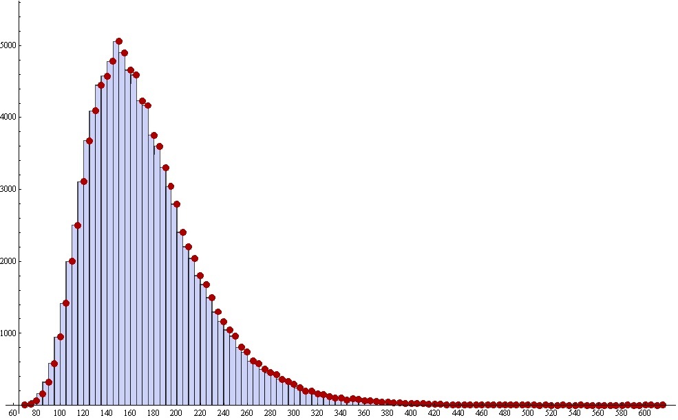
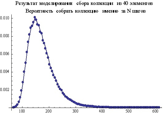
As a result, we get just such a picture. This is a histogram. In it, each column has its own coordinate on the horizontal axis, its height and width. The height of the column indicates how many times out of 100,000 thousand iterations the collection was completed in n steps, and n in this case is the coordinate on the horizontal axis. Roughly, but generally true. And if more precisely, then you need to remember about the width of the column, it is here for a reason. The fact is that when constructing a histogram, the choice of the “adequate” width of the columns is a matter of crucial and complex. When he was chosen and showed you the finished result, you should remember that in fact, the height of the column indicates the number of times events occurred that have a coordinate more than the left border and less than the right edge of the column. Suppose that in principle only integers are possible in our country, and we are going to make 0.25 of stupidity by stupidity. As a result, instead of a “smooth” picture, we get a “comb” from the columns, like a fence with holes — that is, a column, then no, that is, then no. If we take the width very large, then we can get just one very wide column - there will be no sense from it. All bends and nuances will simply be absent.
Now the height of the columns indicates how many times from all the tests the collection was collected in a certain number of steps (gum discoveries). To find out the probability of obtaining a collection at a certain step, we must divide the height of the columns by the total number of tests, and thus, we obtain a numerically modeled answer to the set problem on the collection.
As already mentioned, after a randomly encountered task about the trajectory (see the link above), an idea arose that helped not only to optimize the algorithm, but ultimately to derive the formula.
Each moment of the collection collection process can be described by two numbers: how many unique elements and how many repetitions. The likelihood of receiving a unique element of the collection when you next receive a new element (in the new gum to get an insert that has not yet) does not depend on what elements you already have, but only on how many unique elements you have and how many elements collections.
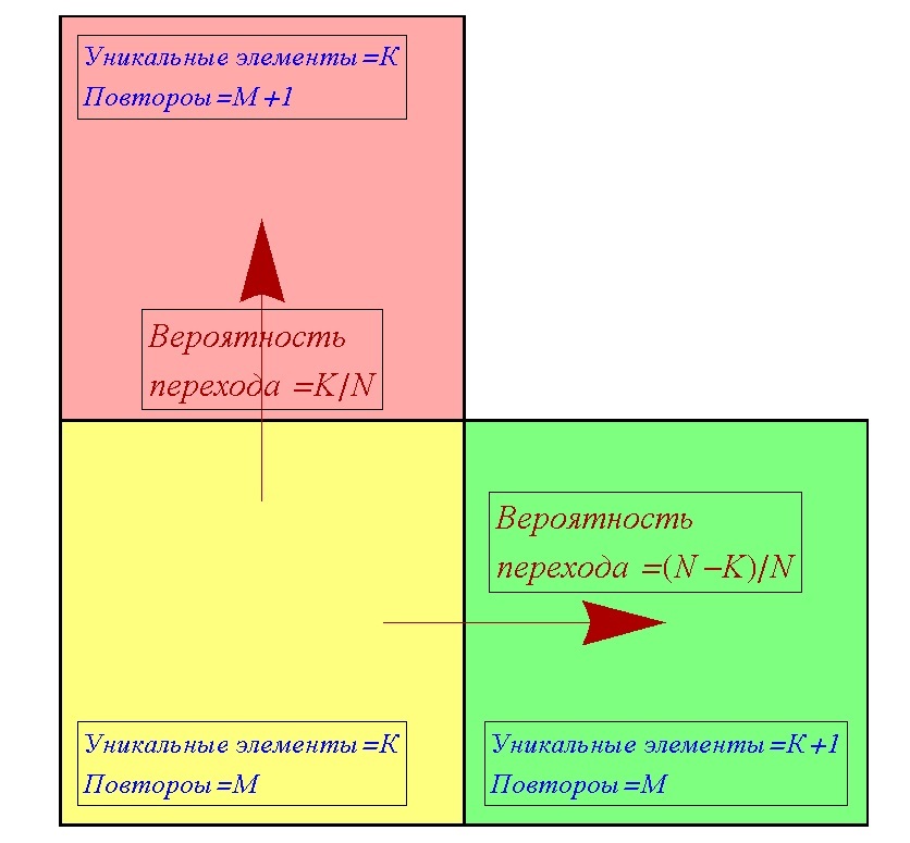
Suppose at some moment there are K unique elements, M repeats, and a total of N elements in the collection. It should be clarified that by the number of repetitions we mean all those elements that will remain with us, if we remove exactly one unique element from the whole of our current set. For example, there are 4 apples, and 3 pears, a total of unique elements 2 are an apple and a pear, and repetitions 7 are 3 apples and 2 pears. When you receive a new item, we can go from the current state (K, M) to one of the two other states. Either we will increase the number of unique elements (K + 1, M), or we will increase the number of repetitions (K, M + 1). Thus, we can build a transition table, for any case (K, M).
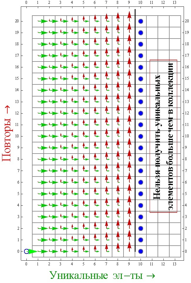
Based on this approach, we can build an algorithm to model the collection collection process. Now we will need at each step with probability (N –K) / N to move either into the cell (K + 1, M) or with probability K / N into the cell (K, M + 1), as long as K < N. When K becomes equal to N, the collection will be assembled, and we will only need to add K and N to find the required number of steps. The probabilities of K / N and (N –K) / N transitions are explained by the fact that the probability of repetition is equal to the ratio of existing unique elements to the total number of elements in the collection, and the probability of obtaining a unique element is equal to the ratio of the number of missing elements to the total number of elements in the collection. It is worth noting that this describes the probabilities of transitions between cells, and not the probabilities of getting into cells (states).
Here is the actual code of this algorithm. It still works faster than the first option.
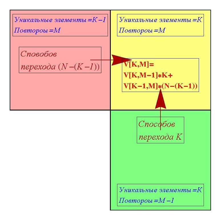
Now we will develop the idea further. You can try to calculate how many options there are to get into the cell with fixed (K, M). The cell (K, M) can be reached either from the cell (K, M-1) or from the cell (K-1, M). Except for cases when we have either only one unique element or no repeats, that is, K = 1, M = 0, they can only be entered in one of two ways. Denote the number of ways to get into the cell (K, M) as V [K, M]. From the cell (K, M-1) you can get to the cell (K, M). To various options, because you can get one more repetition with as many options as there are already unique elements. From the other neighboring cell (K-1, M) one can get into the cell (K, M) (N- (K-1)) by the number of variants, because in the cell (K-1, M) unique elements (K-1 ), and accordingly lacks (N- (K-1)) elements. In general, the options to get into the cell (K, M) through the cell (K, M-1) can be V [K, M-1] * K options, that is, the product of the number of options to get into the (K, M-1) multiplied by the number of options to get from (K, M-1) to (K, M). Similarly, with variants to enter the cell (K, M) through the cell (K-1, M), we obtain V [K-1, M] * (N- (K-1)). In total, you can get into the cell (K, M) with V [K, M-1] * K + V [K-1, M] * (N- (K-1)) by the number of options. Thus, we get the very useful formula for us about the number of ways to enter the cell (K, M).
V [K, M] = V [K, M-1] * K + V [K-1, M] * (N- (K-1))
Using this rule, you can consistently calculate the number of ways to hit for any cell (K, M). That is, it will not be a formula that immediately gives the value of options for specific (K, M), but we will have a table with symbolic answers, and not with numerical simulation. Here is the actual algorithm.
And here is the resulting table, in spite of all its huge size, has a remarkable feature. All columns of the table are proportional with a certain numerical coefficient to the first column. And the given numerical coefficients do not depend on the number of elements in the collection. If we divide all the columns of this table into the first column, we get the following result.
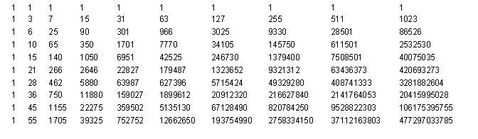
Honestly, I was extremely puzzled when I first got it. It seemed so beautiful and incredible that I just did not fit in my head. These numbers do not depend on the number of elements in the collection and depend only on the number of repetitions and unique elements, that is, on (K, M). If you understand how these numbers are obtained, then the problem will be completely solved and reduced to a very simple formula. But what are these numbers, I did not have a clue.
Imagine that during some calculations, you are faced with a certain coefficient, for example 5.01326. You know that you did not receive it with absolute precision, but you thought, and suddenly this number is some kind of “beautiful” and is expressed through known mathematical constants, or it is the root of some natural number, logo-logic, sine. Well, or if it is not, it is very close to it. For example, such a need can be encountered when analyzing someone else's code, with a list of constants, but without comments. In this case, the Wolfram Alpha website rescued me.
Here is an example of a response to a request for the number 5.01326. (I guess the root of 8 * Pi)
I find it difficult to call Wolfram Alpha a search engine, it is something more. He is not just looking for pages on the Internet, which somehow relate to what you are looking for. It often calculates the answer to your question yourself. And instead of the “bonus” of advertising, as usual search engines do, it gives out really interesting facts related to this issue. Not links, but just the facts on the page. Links, however, also of course gives out at the end of the page, but usually everything that he gives himself is more than enough.
Also, if you wish, you can get access to databases on weather, some financial data, geography, biology, chemistry, and so on. For example, here. Links already with ready requests
Plots of temperature, pressure and other things in Kabul from the 97th to the 99th years.
Information about Apple's promotions over the past 16 years
Map and information about the territory of the USSR
The main properties of nitric oxide
In addition to answering questions like “what is ...?”, He can produce solutions of differential equations entered into the input line. Or draw the graph you asked for. That is, no third-party programs, plug-ins and other things are needed - you can simply solve a differential equation and draw a graph by entering it into the Wolfram Alpha input line. But still, I will note that everything is within reason - if something is rather laborious, he will refuse to be considered “for free”, and Wolfram Mathematica will still be required for complex tasks and speed.
In particular, you can make a request in the form of sequences of numbers, and in addition to the basic characteristics of a given array, it can (not always true) give a presumable option for continuing the sequence. It was this possibility of his that was used to find out what kind of numbers were obtained in the cells above the table described.
Those who do not like detectives can skip this chapter and move on to the next one .
I began by taking the lines of the resulting W array and simply typing it in Wolfram Alpha manually. But you can not copy-paste, but directly from Wolfram Mathematica directly contact Wolfram Alpha without browsers. And immediately request the part of the information that interests. Here is the code that in the loop asks for the presumptive formula of the entered sequence.
Unfortunately, not all requests were successfully processed, the reasons are different, sometimes it helps to reduce or increase the size of the entered sequence. But from the received answers, after a close look, it can be found that the sequences we entered are of the form a0 * 0 ^ n + a1 * 1 ^ n + a2 * 2 ^ n + a3 * 3 ^ n + .... The number of terms is equal to the sequence number of the entered sequence. But the coefficients an are linearly included in the formula, which means that they can be easily found from a system of linear equations. Moreover, if you look closely, all the addends have a common factor inversely proportional to the factorial of the sequence number, and also that the addends are alternating. Therefore, we will look for the terms taking into account these facts. Of course, we solve the system not manually, but in Wolfram Mathematica. Here is the code for the solution.
The coefficients found, but they, too, is not that simple. We repeat with them the same procedure of trying to find a formula for them. And here we are waiting for disappointment - Wolfram Alpha in the freebie mode can not recognize these sequences. Well, try it yourself.
We will try to decompose all these numbers into prime factors and meditate a little, contemplating the result. Such an approach is often useful in recognizing a sequence formula.
Looking closely at the decompositions obtained, it is clear that each of the numbers in the sequences is divided into its own sequence number to a certain extent, and this degree increases with the number of the sequence. Looking more closely it can be seen, this degree is equal to the number of the sequence minus 2. Well, well, then we divide all the numbers in our sequences by their ordinal numbers to the degree of the number of the sequence minus 2.
I did not give the results of the calculation of algorithms before, there are arrays of numbers, and too many tables would have to be inserted. And the numbers, as I said, are not that clear. If someone wants to look at them - then please, I put the code for this. Just run it once and see everything. It will work quickly. This time I will give the result of the algorithm, due to the fact that the numbers are very famous.
{{1}, {1,1}, {1,2,1}, {1,3,3,1}, {1,4,6,4,1}, {1,5,10,10, 5.1}, {1,6,15,20,15,6,1}, {1,7,2,3,35,35,21,7,1}, {1,8,28,56,70, 56,28,8,1}, {1,9,36,84,126,126,84,36,9,1}}
What happened after the division, if you remember Newton's binom and Pascal's triangle, you won't be thrust into Wolfram Alpha anymore. It just turned out "Tse of en ka."
Now it remains to collect all our parts from the disassembled formula back into a single unit.
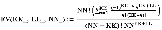
The result is obtained in an analytical form, and in principle, everything you need can be pulled out of it. However, the formula is rather cumbersome, but I would like to make it more compact. And surely it should be known, due to the prevalence of the collection problem.
For a long time I tried to simplify it, or find it in literature. In the end, it turned out to do both after, when, instead of the rows of our source table, I sent to the Wolfram Alpha columns to recognize the sequence.
If you enter the columns of the resulting W array in Wolfram Alpha , the sequence will be recognized as Stirling numbers of second kind. This is a fairly well-known (as it turned out, although I did not remember them / did not know) array of numbers, which is described in detail in various textbooks on combinatorics and probability theory. Those who are familiar with Stirling numbers can skip this chapter and move on to the next one .
You can read about the Stirling numbers, for example, here .
And here it is much more detailed , but, really, in English. It is, in general, perhaps one of the best sites if you need complete background information about something from mathematics.
The second-kind Stirling numbers mean the number of ways to split a set of N elements into K parts. For example, the set {1,2,3,4} of the four elements can be divided into:
into 4 sets by one element, {{{a}, {b}, {c}, {d}} (only one way)
into 3 sets , where in one there will be 2 elements in the remaining {{a, b}, {c}, d}}, {{a, c}, {b}, {d}}, {{a, d }, {b}, {c}}, {{b, c}, {a}, {d}}, {{b, d}, {a}, {c}}, {{c, d}, {a}, {b}} (total 6 ways)
into 2 sets of 1 and 3 elements {{a}, {b, c, d}}, {{b}, {a, c, d}, {{c}, {a, b, d}}, {{d}, {a, b, c}}, or 2 elements each {{a, b}, {c, d}}, {{a, c}, {b, d}}, {{a , d}, {b, c}} (there are 7 ways)
On 1 set of 4 elements, that is, without breaking anything. (only one way)
The actual number of ways to partition the set into a certain number of parts (but at the same time, an arbitrary composition of these parts) also denotes Stirling numbers.
James Stirling, a Scottish mathematician, lived about 300 years ago, a contemporary of Isaac Newton, with whom he regularly corresponded, communicated, and worked. Numbers denoting the number of ways to split the set into n parts are named after him.
The formula for obtaining the Stirling numbers of the second kind is as follows.
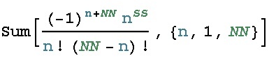
But in Wolfram Mathematica they are available through the StirlingS2 [SS, NN] function.
The task of a collection of N elements can be solved in three lines. True, in order to understand this, it took me quite a lot of time.
Thus, the probability of collecting a collection of K elements in N steps is equal to StirlingS2 [N, K] * K! / N ^ K
Those who are familiar with the concepts ":" The distribution of a discrete random variable "and" and "The distribution function of a discrete random variable" can skip this chapter and go on to the next .
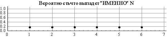
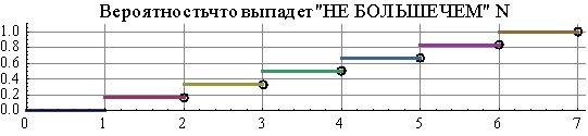
Let us roll the dice. The probability that a given specific number will occur, for example, 3 or 5 is 1/6. The graph of the probability of these events is just a horizontal line, well, or let us call it a “shelf” (it looks like it). But very often there is another question. What is the probability that a number will fall out less than or equal to a specific given number, for example, less than or equal to 2. Then for each of the possible numbers you can also build a probability graph, but it will already be in the form of a “ladder” and not a horizontal line like the last time.
Moreover, as we see, there are no values for 3.5 or 2.8 points on the “shelves” graph, simply because you will never throw them out with a cube. In this case, whether it is necessary for non-integer numbers, or for those that are less than one or higher than 6, consider the probability to be zero or be considered uncertain - the question is rather complicated, but for the time being we will simply bypass it. As for the "ladder", there is also an important point, which is not difficult to understand, but it is very easy to skip it and make a mistake as a result. The horizontal part of each step “has a point on the left border”, but “has no right”. In the sense, you can get as close as you like to the convex corner of the stair, but the value of our ladder function in the place where the graph breaks occur is equal to the value of the upper (next) stair. For example,the probability of getting a number less than or equal to 2 on the dice is 1/3, the probability of getting a number not more than 2.5 is also equal to 1/3, the probability of getting a number not more than 2.999999999 ... is also equal to 1/3, but the probability of getting no more than 3 is already 1 / 2
The cube is the same. It seems like there and there we build a probability graph. But they are different. Very often, when studying a terver, problems arise precisely because of the confusion of these two entities. This is partly due to their names, which are very similar. And partly with the fact that it is not entirely clear why they were introduced by two, it was possible to do with one. Especially the “ladder” is initially perceived as weakly informative and meaningless.
These two entities are called so:
Now, if someone has a clear and understandable ear for the striking difference between “function” and “law” - eat a cookie. It is especially bad when, during a conversation, the “distribution function” is simply reduced to “distribution”, and that’s all, hello, there is simply no difference. It's a shame that there is a misunderstanding of important things, as it turns out, only because of the linguistic jambs, and not because you are not able to understand the meaning. The teachers on the terver do not see any problems here, but the students suffer.
It is clear that the "shelf" and "ladder" are not always so obtained. For example, if we were drawing a graph not for the values of the cube, but for the growth of people, then the graph would no longer be a shelf (people are not all the same height), but rather some kind of “dome”. The maximum of it would be somewhere probably 160cm. but the probability of growth of 200cm as well as 140cm would be much lower. The ladder, however, in the discrete case, most often it is the “ladder”, (we do not consider the cunning rare cases now, because of their impracticality), but still, this ladder is usually quite uneven.
It is best to perceive these entities in the head abstractly, without a name. But in a conversation, it is necessary to apply something concrete and not an abstract one - therefore, I usually (although of course the Terverschik will bury me alive for this) apply the following concepts. "Integral" to denote the essence of the "ladder", and "density" to denote the essence of the "shelf". Such definitions are quite well within the meaning. The probability that a number less than or equal to three falls on the cube means the sum of the probabilities that 1 drops out or 2 drops out or 3. That is, the sum of the probabilities of all possible options less than 3 will give values for the “integral” - “ladder” graph at point 3. The integral is, in fact, the sum, hence the notation I use. Density is, to say simply and roughly, the mass of one small piece of the total volume. When,when we talk about the probability of a strictly fixed single value falling out, we, as you isolate from the whole set of possible values, only him, alone, and talk about him. From here and the second used designation.
Now the question remains - why do we need to separately enter such an entity as a graph of the "integral" -probability. For a cube, this is really not very clear. Let's try another example. Suppose we have a hundred people, each of them receives a salary, which depends on the length of service, various merit in work, qualifications, etc. In this situation, all the salaries will be at least a little different. One gets 30t.r. another 32, five people are 35, some 36, and exactly 34 nobody gets, and so on. Now imagine that you have a “density” -probability graph, that is, from it you can say that the probability of getting exactly 32t.r is equal to 1/100, and the probability of getting 34 tr. do not understand what (we have 100 people, and only one gets 32t.r, and 34 no one gets).Well, what useful conclusions can be drawn from the knowledge of the probability of 1/100 for 32t.r or from the fact that there is simply no data for 34t.r? Essentially no. Now imagine that you have a graph of the "integral" -probability. According to it, you can say what is the probability of receiving less than 30 rubles, and this will be a significant percentage. And if for example the probability of less than 10 tons. P turns out to be zero, then this means that no one gets less than 10 tr, which is much more informative than the fact that the salaries are 34,234 rubles. 20k no one else has.then this means that no one gets less than 10 tr, which is much more informative than the fact that salaries are 34,234 rubles. 20k no one else has.then this means that no one gets less than 10 tr, which is much more informative than the fact that salaries are 34,234 rubles. 20k no one else has.
Of course, you can even come up with graphics like "the probability that more than something and less than something," then the amount will not go for all values less than the specified, and from one value to some other. But these are concrete examples, which are specific for each specific case. But the graphs of "probability-integral" and "probability-density" are widely used by all, therefore, they are divided into two separate important entities.
Understanding the meaning of these two entities, as well as an understanding of the appropriateness of their use are needed in order to comprehend the formulas for the collection problem that we received, as well as the data that we obtained in numerical simulation. This is how the probability graph of collecting a collection looks for a certain number of steps depending on the number of steps, and I also remind you once again how the data obtained by modeling looks. Charts vary greatly.

The difference is explained by the fact that the graph obtained by modeling is “density-probabilities”, and the one that by the formula is “integral-probabilities”. The formula gives the probability value to collect the collection in N steps. Not exactly for N! And simply - for N. That is, we could collect the collection almost immediately, and then we would only get repeated items until we took N steps, and we still took into account such a strange case in our probability. So that there is no confusion or misunderstanding, then it’s better to say about our formula “The probability of collecting a collection in N or less steps” or “... in no more than N steps”. And about the graph obtained by modeling you need to say, “the probability of getting the collection exactly at the Nth step”, that is, when at the (N-1) -th collection was not collected yet, but at the Nth step it was collected.
To get the formula for "density-probability" from the formula for "integral-probability", you need to collect the collection in N or less steps from the probability to subtract the probability to collect the collection in (N-1) or fewer steps. The resulting difference will be the probability to assemble the collection at the Nth step, and not earlier. Thus, the probability of assembling a collection of K elements exactly at the Nth step is equal to StirlingS2 [N, K] * K! / K ^ N- StirlingS2 [N-1, K] * K! / K ^ (N-1)
It is worth noting that this formula can be reduced. The fact is that when it remains to collect only one element, this can be done in only one and only one way. This means that the probability of collecting a collection at the Nth step is equal to the ratio of the number of opportunities to collect it in (N -1) steps to the total number of all possible elements in the Nth step. As a result, the formula is reduced to the form of StirlingS2 [N-1, K-1] * K! / K ^ N
In the following graph, the formula for collecting the collection is shown on the Nth step as a solid line, and the red dots indicate the simulation results. As you can see, they match up pretty well.

What is now being described is extremely important and useful to know in everyday life. Those who are familiar with the notion of mean, expectation and median may skip this chapter and move on to the next one .
Often the question arises: how many “on average” do you need steps to assemble a collection? It seems to be a simple question, natural, often encountered, but there is one problem. It is necessary to clarify what exactly we want to know when talking about the "average".
Imagine such a situation, the seller, every day makes a profit in the amount of one, two, three, and so on up to 6 thousand rubles. As if his daily profit depends on the number that fell on the die roll. And after a month of work in this mode, he decided to calculate the average. Calculated the amount of profit for all thirty days and divided by the number of days. The resulting number is the arithmetic average of the profit for all 30 days. The number is quite informative, but it has one significant disadvantage-lack. The fact is that it can be calculated only if you already have information about some of the events that have occurred. If he wants to find out the average value of profit for the next month, then he cannot find it out using the arithmetic average calculation method now, at the moment he cannot - he has no data for the next month yet,which could be folded and divided. But, his work next month, it seems, will be the same, no cataclysms are foreseen, he also does not expect interruptions in the supply of goods and a drop in demand. The seller expects that next month the properties of a random variable will not change. Well, if so, then we can assume that the average value that he will be able to calculate in a month will also not differ much from the average that was obtained last month. The question of what “not much” means, we will skip for now, it is rather complicated and not very relevant now. Let's better try to find a way to predict the approximate average profit in the next month.he also does not expect interruptions in the supply of goods and a drop in demand. The seller expects that next month the properties of a random variable will not change. Well, if so, then we can assume that the average value that he will be able to calculate in a month will also not differ much from the average that was obtained last month. The question of what “not much” means, we will skip for now, it is rather complicated and not very relevant now. Let's better try to find a way to predict the approximate average profit in the next month.he also does not expect interruptions in the supply of goods and a drop in demand. The seller expects that next month the properties of a random variable will not change. Well, if so, then we can assume that the average value that he will be able to calculate in a month will also not differ much from the average that was obtained last month. The question of what “not much” means, we will skip for now, it is rather complicated and not very relevant now. Let's better try to find a way to predict the approximate average profit in the next month.which means “not much”, we will skip it for now, it’s rather complicated and not very relevant now. Let's better try to find a way to predict the approximate average profit in the next month.which means “not much”, we will skip it for now, it’s rather complicated and not very relevant now. Let's better try to find a way to predict the approximate average profit in the next month.
When we considered the arithmetic average, we summarized all the values obtained during the observations of random values (wages) and divided by the total. Let's look again more closely at this whole process. Let's write all the data in the table.

The unit fell k1 number of times, two k2 times. (We have been counting there in thousands, but for brevity we will not write zeros). After that, we found the sum of everything that fell on the dice (well, or whatever it was - earned in a day). The terms of this sum were the numbers 1 2 3 4 5 6, with 'each of them, respectively, k1 k2 k3 k4 k5 k6 times. And this means that this sum is equal to S = k1 * 1 + k2 * 3 + k3 * 3 + k4 * 4 + k5 * 5 + k6 * 6. The total number of terms in this sum was N = k1 + k2 + k3 + k4 + k5 + k6. After all, k [x] denotes how many times each of the values falls, and a total of 6. Then we divided S into N, which is S / N = 1 * (k1 / N) + 2 * (k2 / N) + 3 * (k3 / N) + 4 * (k4 / N) + 5 * (k5 / N) + 6 * (k6 / N). But if you look closely, then k1 / N is very much like the probability of a unit falling out, respectively, k2 / N is the probability that two will fall, and so on. Indeed, wewe divide the number of the occurrence of an event by the total number of events. But the process of dropping random numbers, the very law of the distribution of random values did not change last month and did not seem to change in the following. This means that relations like (k1 / N) do not depend on time, but depend only on the properties of a random variable. And if one day we can get them from observations obtained experimentally, (and of course, counted and divided), then we can use them in the future. Moreover, it turns out that S / N now also depends only on the properties of randomly magnitude and does not depend on time, it now only contains terms of the form WHAT_ EXTRACTED * PROBABILITY_PUT-OFF_ THAT_THE_READ.the distribution law itself didn’t change in magnitude last month and didn’t seem to change in the following. This means that relations like (k1 / N) do not depend on time, but depend only on the properties of a random variable. And if one day we can get them from observations obtained experimentally, (and of course, counted and divided), then we can use them in the future. Moreover, it turns out that S / N now also depends only on the properties of randomly magnitude and does not depend on time, it now only contains terms of the form WHAT_ EXTRACTED * PROBABILITY_PUT-OFF_ THAT_THE_READ.the distribution law itself didn’t change in magnitude last month and didn’t seem to change in the following. This means that relations like (k1 / N) do not depend on time, but depend only on the properties of a random variable. And if one day we can get them from observations obtained experimentally, (and of course, counted and divided), then we can use them in the future. Moreover, it turns out that S / N now also depends only on the properties of randomly magnitude and does not depend on time, it now only contains terms of the form WHAT_ EXTRACTED * PROBABILITY_PUT-OFF_ THAT_THE_READ.(well, of course, counted and divided), then we can use in the future. Moreover, it turns out that S / N now also depends only on the properties of randomly magnitude and does not depend on time, it now only contains terms of the form WHAT_ EXTRACTED * PROBABILITY_PUT-OFF_ THAT_THE_READ.(well, of course, counted and divided), then we can use in the future. Moreover, it turns out that S / N now also depends only on the properties of randomly magnitude and does not depend on time, it now only contains terms of the form WHAT_ EXTRACTED * PROBABILITY_PUT-OFF_ THAT_THE_READ.
Let's not write a lot of words, we denote all the possible options TOGO_CHOUCHALO through X (i). (“X and i'm - meaning as the fifth, sixth, entho, katoe, itoe”) In total, we have X (i) six pieces, since our random variable takes only one of six values. Moreover, X (1) = 1, X (2) = 2 and so on. AND THE PROBABILITY_FALLS_TOTTEN_OURSELVES through P (i). And to each value of randomly the values of X (i) there corresponds its own probability of P (i) falling out. In such designations, the S / N value can be written more simply S / N = Sum All [P (i) * X (i)] (for all i). We have only 6 pieces, we will write them out for clarity.
S / N = P (1) * X (1) + P (2) * X (2) + P (3) * X (3) + P (4) * X (4) + P (5) * X (5) + P (6) * X (6)
So here.The value SumVseh [P (i) * X (i)] (for all i) is called the expectation value . In the sense that it is not yet obtained, but expected after mathematical analysis, the average value of a random variable. For a die, the expectation is 1 * (1/6) + 2 * (1/6) + 3 * (1/6) + 4 * (1/6) + 5 * (1/6) + 6 * (1 /6)=21/6=3.5. For a cube whose faces are only integers, it is usually not easy to understand what a 3.5 is when you first get acquainted with this fact - there is no 3.5 face! And the expectation mat at all should not be equal to one of the values of the random variable. For our seller, who receives an average of 3500r profit per day, everything is pretty clear.
Now imagine that you threw a cube 10 times, and all 10 times it had the number 6. If you calculate the arithmetic average value, then it will also be 6 (well, obviously). And we say that mate. expectation of 3.5, and that exactly 3.5 should be an average value, and not like 6. It is here that we see that the arithmetic average value obtained from the observed data may differ from the expected value. And in general, the expectation is the expectation of an average, and not something that can sometimes happen in reality. Expected, close to reality, but not equal to the real value of the straight for sure. However, there is a theorem (“The Law of Large Numbers”), which says that the more times we roll a cube, and for all these times we calculate the arithmetic average, the smaller will be the difference between expected value and average value. And consideringthat in most cases we have no opportunity to conduct long experiments, and indeed, it would be desirable to predict without any experiments what happens there “on average”, then we need to be content only with using mathematical expectation, as some estimate, prediction with some kind of error.
On the one hand, the average value is quite informative when describing some random processes, but sometimes, the average value is simply meaningless, illogical, and its use is contrary to common sense and reality. And the matter is not in the very mean, but in the sanity of those who consider it.
The head physician of one of the hospitals liked to write the following wording in the reports: “The average body temperature of the patients is 36.6 degrees, which fully corresponds to the norm”. He did not lie, but honestly considered the temperature of all patients, and those who had a fever of 40 degrees, and those who died and cooled to room temperature. On average, it was 36.6. It would be much more informative to draw a graph of the temperature distribution of patients, looking at which, it would be possible to estimate how many people are still alive, and how many of them have a fever above the norm, which means you need to throw all your strength on their salvation. An example, of course, anecdotal, but bright, about what to read the average value is sometimes meaningless.
Another example of the use of the average value, is not even so much senseless as harmful, and misleading people. Often in the media you can hear a mention of the average salary in a certain industry. The schedule for the distribution of wages is usually no one shows, or too lazy to print, or laziness from the extras to ask him. And I will show you (made up of course, but very close to reality).
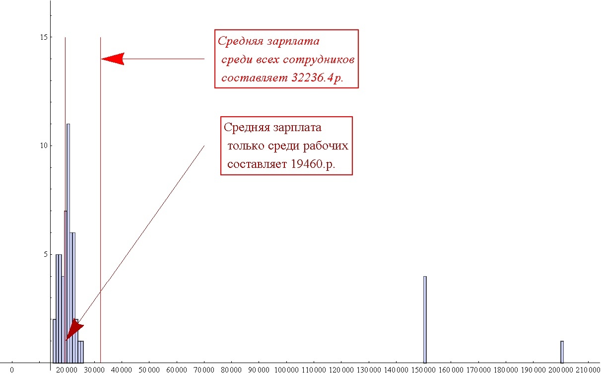
Here is the distribution: 50 workers receive approximately 20t.r. the chief of 200, and his four deputies of 150t.r. The media honestly writes that the average salary at this enterprise is 32,236 p. And 40 kopecks. The workers, of course, are very surprised when they hear that it is on average that they receive such a salary. The average value is exactly that. Only it is one and a half times higher than the salary of most employees. And now no one has ever deceived anyone. On the other hand, it would be more correct to show the graph, but much longer. And the graphics are quite complex, and not everyone will immediately understand what is depicted on it. Yes, even in our task about the collection, I am more than confident that not all people will want to look at, or even more, build the graphs themselves. Rather, they will want to hear the very "average" number of items to collect the collection.One number is somehow easier to grasp than a distribution.
There is one more “number” which briefly, but sometimes more informatively describes the distribution law, than the expectation. It is called the median (no, this is not the median of the triangle, just the names are similar).
In the previous example about salaries, you can ask this question - no more than what amount do 50% of employees receive. This is the sum that will be the answer to this question and is called the median. However, the median does not always exist, but there is some value nearest to it. This nuance does not play a special role, well, you can not get a value strictly for 50%, but the closest, it is always possible. In this example, we can say that 61.8% of employees receive a salary of no more than 21 tons. Moreover, we can say that 89% of employees receive a salary of no more than 25t.r. This number will not be called a median, but a quantile (89%). In fact, the median is also a quantile, but because of its frequent use and because it is exactly 50% percent, she was given her own name. Agree, the phrase “89% of employees receive a salary of no more than 25 tr."It sounds much more informative than the" average salary of 32 tr. " Ideally, of course, it is better to say this and that, not too long or hard to say. True, listeners may be unaccustomed and don’t understand what they said to them.
Particularly thoughtful will probably ask, and what exactly 50% we will take, and if the chief with the deputy enters these same 50%, then again it will turn out nonsense. Yes, it turns out, so you need to first sort all by ascending, and count the percentages from minimum to maximum. I missed this moment in the description of the law and the distribution function, but they are always built precisely in ascending order.
In practice, quantiles, or even the median, can be quite difficult to calculate. For the median, it is necessary to solve an equation of the form F (x) = 0.5, and the inverse function is far from every distribution easy to calculate, and it does not always exist, and therefore it is necessary to look for the nearest one. As a result, we will not get an equation, but an inequality, and if we then need quantiles for different cases (for different enterprises or months), we need to write and compare, and we will have them from different percentages, then it will be inconvenient.
For the collection problem, by the way, I don’t know how to calculate the quantile analytically, but we get it by numerical solution.
In the collection task, I would like to know how many collectors, on average, take steps (open the gum) before they collect the collection. You can use the formula for mathematical expectations and use the law of probability distribution (the one that is “density”) that we obtained earlier. But I must say I could not calculate such a sum - the formula is still quite complicated, and how to roll it is not clear.
If it is impossible to solve it “in the forehead,” we will try to at least somehow. One of the properties of mathematical expectation will help us in this. I will give it without proof, which is short and not complicated and can be found in any textbook on the Terver.
Mat expectation of the sum of two independent random variables is equal to the sum of the expectation mat of each of these variables.
For example, a die cubic. Expectation 3.5. And what is the mathematical expectation of the sum of the numbers on two simultaneously thrown dice. According to the above rule, we get the answer 7.
Suppose at some point we have K unique elements, and in total there are N elements in the collection. The probability of getting another unique element is (NK) / N, and the probability of getting another repeat is equal. K / N. In such a situation, the probability of obtaining a unique element in exactly M steps is equal to (NK) / N * (K / N) ^ (M-1), that is, it is the probability of obtaining a unique element provided that before this we only received repetitions. To calculate the average value of the steps that need to be done to obtain a new unique element, we use the formula for the mathematical expectation. It is by the way not difficult to be considered manually, but here is the code for calculating in mathematics.
As a result, we get that if we already had K unique elements, then on average we need to take N / (NK) steps (open the gum) to get a new element.
The average value of the obtained elements (all open chewing gum) to collect the entire collection is equal to the sum of the average values of the number of steps that was made between obtaining unique elements that are equal to N / (NK). For example, in order to get the first unique element you need N / (N-0) = 1 step (opening the bubble gum), in order to get the last unique element you need on average N / (N- (N-1)) = N steps , for the penultimate N / (N- (N-2)) = N / 2 steps, for the penultimate last / N / (N- (N-3)) = N / 3 steps and so on. As a result, we get the sum of this type N + N / 2 + N / 3 + N / 4 + ... + N / (N-2) + N / (N-1) + N / N. Which can be written in a simpler form: N * (1 + 1/2 + 1/3 + 1/4 + ... + 1 / N).
This is the answer to the question of how many on average you need to get items to assemble a collection .
Do not even try to enter the Russian Wikipedia. Everything that concerns formulas, theorems and something a little bit scientific on Russian wikipedia is harmful to watch! The articles are scarce and written in such a language that it is simply not realistic to learn something from them. It seems that having wiped out pieces of definitions from the middle of fairly serious books written using the most non-obvious symbols, the authors of Wikipedia articles simply copy-paste them, without trying to explain the essence of the question or at least the meaning of the notation used. And not rarely with significant semantic errors!
Most users have already formed the opinion that everything is written quite simply on Wikipedia, and if this is so, then if it is not clear on Wikipedia, then the question is extremely complex and it is better to forget about it. Some kind of anti-textbook is right - instead of being interested and enlightening, it pushes them away from studying completely or is misleading.
By the way, in the process of searching for questions related to the topic of this article, I was brought to the Wikipedia page dedicated to James Stirling .
He lived 300 years ago, and the image that is attached to the page made me suspicious because of the quality of the image and the appearance of the depicted man. On the pages of James Stirling in other languages, this image was not everywhere. In most cases it was not there, but it was present on the pages in Slovak, Armenian, Hungarian, Hebrew and Russian. The link to the image gave a very interesting result .
It turns out that this is a photo of Gustav Bergman, a philosopher of the 20th century. At least on the official website of the University of Iowa this is stated.
Once Wikipedia contained really good, reliable articles, but everything changes. And the Russian Wikipedia continues to change for the worse.
But in fairness, I note that the English Wikipedia pages are often well written.
Formulas that can be written using Stirling numbers of the second kind will be written in two versions.
Since the letters N and K are reserved in Wolfram Mathematica, designations of the form NN are used. This means one character, not the product of two characters.
In all formulas, NN denotes the number of elements in the collection, KK - the number of unique elements, LL - repetitions. Sometimes there will be MM - it means all the elements that are available at the moment (what the collector now has). Yes, MM = KK + LL, and the introduction of this notation seems redundant, but it is convenient when describing a formula.
Some formulas come in two versions using StirlingS2 and in general. But these 2 options are completely the same.
In the game ArcheAge in hard-to-reach places on the western mainland, you can find the “Traveler's Bag”, in which, among other things, there will be pages from Eric's diary. If you collect all 80 unique pages, you can restore a complete diary from them, and as a reward you can get a title that gives the holder the ability to receive less damage when falling. Using the formulas obtained, we can say that on average, a player needs to find 397 bags in order to independently collect the entire diary. You can also say that picking up 400 bags, the probability of collecting all the pages is 58.7%.
Sometimes, and maybe even often, people rather recklessly rely on their intuition, not devoting the proper time to the mathematical analysis of questions. I suggest you (and then you can offer your friends) to answer two questions. Try to answer them, relying only on your “inner feelings” on your intuition.
The first question is this. There are 23 pupils in class. What is the probability that at least one of them has birthdays?
The second question is about mold. One cell of a mold flew into a jar with a nutrient solution, and in time t was divided into two. After that, each of these two cells was again shared in time t. After 1 hour, the jar was filled exactly half the mold cells. How long does the bank fill up completely?
Wait, do not read further, try to still give at least some answer, imagine that if you answer correctly you will get 1000r, and if it is not right then 100r, and if you don’t answer in a minute, you will not receive anything. It's just for an incentive, but now you will think that the problem with the trick is that you need to “think”. And people usually begin to carefully analyze only when they begin to suspect a trick. Which, of course, is good. But it would be good not to rely on intuition in other cases. However, it is now that your test of your intuition. Have you answered?
The answer to the question about birthdays in one line is obtained from the previously derived formula about the collection. All days in a year are the number of items in the collection, 23 people are the current number of items you have, repetitions are 0. The probability that at least two people have birthdays is the same is one minus the probability that birthdays do not match no one. And in terms of liners and chewing gum, this means 23 unique elements, 0 repeats, and 365 elements contains the entire collection. We get that the probability of coincidence of birthdays in at least two of 23 people is
1 - FV [23,0,365] = 0.507297 = approximately 50%
That is, in your class, someone's birthdays coincided with a rather high probability. In our class, by the way, it was exactly my birthday that coincided with one of my classmates. As practice shows, for most people, regardless of the type of activity, such a high probability is rather unexpected. For example, I was very surprised to find out the answer. But the truth is then glad that the formula about the collection works very well here.
The answer to the question about the mold, I suggest to find you yourself.
Intuition, excitement, emotions without all of this would be quite boring to live. But, nevertheless, these are the weakest points of man. And it is precisely these weak points that fraudsters, advertisers, PR managers, marketers, many who are actively beating. Mathematical analysis of the information received and your own plans can be either an excellent defense or a powerful weapon. How to apply it is up to you and your conscience. The main thing is to develop the habit of mathematical analysis of the information received in all situations, from going to the store, reading the news to planning tactics and strategy during computer games. Especially during the games.
Introduction
When it remains to get only three of the hundred items in order to collect the entire collection (inserts of BomBimBomb gum or Turbo, or a set of heavy armor for a computer game character), then the fire in the eyes and waiting for a miracle suppress both logic and intelligence and mathematical analysis from the head completely . There is only one thought “A little bit more and I’ll get the rest! I will collect all! At this time, relatives and friends of this obsessed collector are puzzled with only one question - “Oh, a little bit, how much ?!”. How many mothers need to buy more hateful chewing gums, or how many more girls need to sit alone, until her boyfriend knocks out the “most rare pants of Baal” from monsters ?!
Answering the question “how much to buy chewing gum to assemble a complete collection of N-pieces of inserts” is quite difficult at once, even if you use Yandex, because it is difficult to formulate the query itself for an “ordinary” search engine. Attempting to solve the problem yourself usually puts people at a dead end - it’s not clear which way to approach it.
This article will address three questions: How to approach tasks that are not clear at first glance how to solve? What search engine to use in order to receive scientific answers to scientific questions (and not to receive offers to buy a quadratic equation on eBay)? And of course, how much does one need to buy chewing gum to assemble a collection of liners?
Article Navigation
The article was quite large. Therefore, in those places where you can miss something, I will report about it. In such chapters will be considered not the solution of the problem, but those concepts and principles that are used when solving it. If the details become interesting, you can re-read the missing places later. The wording of the task should be reviewed, but further, those who want to get acquainted with the answer as soon as possible can go directly to the results. I advise, however, separately to familiarize with the chapter devoted to Alpha Wolfram .
Also for convenience, I cite a complete list of chapters.
- Formulation of the problem
- Boys, girls and balls
- Mathematical modeling of an obsessed collector
- Curious table
- I am Alpha Wolfram
- Math Detective
- Three hundred years ago
- Three lines
- Two entities
- The average temperature of patients and the average salary of doctors
- Where not directly climb, we will go sideways
- Some kind of wiki
- results
- Birthday and pot mold
- findings
')
Formulation of the problem
To make it clear to those who love mathematical rigor, and to those who are not familiar with it, I will formulate the collection problem in two ways.
- (Through a language familiar from childhood) Let each gum contain one of K liners with equal probability. What is the probability that buying N chewing gum, we will collect the entire collection of liners (we will have K unique liners)?
- (In a more scientific language) Let a set of K elementary outcomes be given (all outcomes are equiprobable). What is the probability that after N experiments performed, each event will occur at least once?
We will immediately clarify a number of points that will further help us in the decision. First, for simplicity, all elements of the collection will be numbered from 1 to K, and thus simply deal with numbers. Secondly, our elementary outcomes will be sequences of numbers of length N, consisting of K different numbers. For example, if K = 3 and N = 5, then the sequences {3,3,1,2,3}, {1,2,3,3,3}, {3,3,1,1,1} are one of possible outcomes, and the order of the elements matters. If in such a sequence all K numbers occur, at least once - this means a “successful” sequence for us, if it does not occur, at least one number never, then the sequence is not successful for us. Moreover, any possible sequence is equally probable. Thirdly, we can always count the number of all possible sequences of K numbers, the length of N elements, provided that the order matters. This number is K ^ N. Fourth, the probability of collecting a collection in N steps is equal to the ratio of "successful" sequences to the total, that is, to K ^ N. Thus, it is possible to search for either the probability or the number of “successful” sequences - as it will be more convenient, one can always be obtained from the other.
Boys, girls and balls
Those who have no questions about "order matters" and "quantity is K ^ N", as well as who remembers what "factorial" and "C from n to k" are, you can skip this chapter and go on to the next one . For those who have thoroughly forgotten combinatorics, or have not yet been acquainted with it, consider the main points that will be useful to us.
The history of combinatorics, though rooted in deep antiquity, still actively developed thanks to gammers. Well, maybe Cardano, Galileo, Farm Pascal and the rest of the great minds of the world themselves were not avid gamers (though not a fact, not a fact), but at least their gamers specifically bothered with questions about games, about winning strategies, asked for guides to write. Of course, then more than dice and cards were played, gambling fans with tanks or magic were somehow not very many. With one there was a shortage, and for the other burned. But actively applied to the analysis of puzzles and gambling, combinatorics was extremely useful for solving practical problems in almost all branches of mathematics. In addition, combinatorial methods have proven useful in statistics, programming, genetics, linguistics, and many other sciences a long time later. Wikipedia EVIL (I’ll remember this more than once), but reviewing things not related to formulas is physically possible to read there, but you shouldn’t trust them. Nevertheless, you can read the article "History of combinatorics"
While I was looking for various materials on combinatorics, I came across a site , or rather, one of the documents from this site. I liked the language with which it is written, you can get acquainted with the combinatorics there. I, in general, would not have remembered this site, if not for one “but”. There is a problem about the trajectory. I liked it very much, it seemed interesting, and looking at it, I had an idea how to solve the problem about the collection, but more on that later.
Here are the basic facts from combinatorics, which will be useful to us.
1.) What is the total number of N -digit numbers in the number system with base K? In how many ways can representatives of K nations be placed on the N chairs? How many ways can you color N squares if there are markers of K different colors? In how many ways can you fill N boxes with multi-colored balls, if the number of different colors K and only one ball fit into each box?
The answer to all these questions is one - “Accommodation with repetitions”. In the case of balls, in the first box we can put a ball of any of K colors. That is, we have K options to shove one ball in the first box. In the second box we can also shove the ball in K ways. The options for filling the first and second boxes with balls will already be K * K = K ^ 2. This happens because for each option of filling the first box there can be any of K options for filling the second box. If we have N boxes, then the options will be K ^ N.
2.) How many there are N -digit numbers in the number system with the base N, such that each digit in the number occurs exactly once? In how many ways can representatives of N nations be placed on the N seats, so that a representative of each nation sits? How many ways can you color N squares, if there are markers of N different colors, so that each marker can be used (without repainting, of course)? How many ways can you fill N boxes with N numbered balls?
The answer to all these questions is one - "Rearrangement". Cases with balls and numbers, in general, are identical, even in their wording. In the first place we can put any of the N balls. On the second place is any of the remaining N-1 balls, on the third one of the remaining N-2 balls after filling the first two places. And so on until the last. It turns out that we have the product N * (N-1) * (N-2) * (N-3) * ... * (N- (N-2)) * (N- (N-1)). Here is the product of all natural numbers from 1 to N and is called factorial. And it is designated as “N!”. Yes, an exclamation mark, this is the designation of factorial or product of all natural numbers from 1 to N. It is extremely common everywhere, and considering that writing it in the form of a work for quite a long time, we decided to simplify and shorten the record to the exclamation mark icon. There is an old joke about factorial that teachers love to tell.
At the matane exam, the lecturer asks the student to expand the exhibitor into a Taylor series.
Student: One plus X divided into ONE (pronounces loudly and solemnly) plus X in the square divided into TWO (also loudly) plus X in the cube divided into THREE
Lecturer: Okay, okay, it's all right, just why are you screaming like that ?!
Student: Well, the exclamation point is the same !!!
It should be noted that the factorial from zero is 1. 0! = 1
3.) In how many ways can K boxes be filled with numbered balls? (balls more than boxes) You have N movie tickets and K girlfriends. How many ways can you hand out tickets to your friends? (there are more tickets than friends)
The answer to these questions is “Accommodation WITHOUT repetition”. However, the decision is similar not to the first point, but to the second. In the first place we can put any of the N balls. On the second place is any of the remaining N-1 balls, on the third one of the remaining N-2 balls after filling the first two places. And so on until the drawers run out. So, the product will be N * (N-1) * (N-2) * (N-3) * ... * (N- (K-1)). That is, the product of all natural numbers from K + 1 to N. But such a product can be painted as N * (N-1) * (N-2) * (N-3) * ... * (N- (K-1)) * (NK)! / (NK)! = N! / (NK)! That, in general, is significantly shorter.
4.) The last point is about why order may or may not matter. And what is "C from n to k".
Suppose you have a UAZ, and you are going to go with friends (only guys, without girls) for fishing. In the UAZ can climb K people. And all in all you have N. friends. Anyone who does not fit into your UAZ will drive other cars. How many options are there to fill in your friends with UAZ? How many ways are there of 20 (N) of your friends who are now online to assemble a team of 5 people (K) in order to play dota for an hour? (Of course there is a nuance - to consider you or not, but we will not bother with it)
What is the difference of this example from all previous ones? That order does not matter. Who, how and where will sit in the UAZ, or who you are first, and who will call the second to the team, no matter what role. The main thing is the composition, and who is where it is no longer important. If order were important, it would be exactly the previous version, that is, the answer would be N! / (NK) !. But order is not important to us. And about the order we had an example 2) with factorial. That is, N! / (NK)! must be divided into K !, and then the cases, which differed only in sequence, but were identical in composition, “would collapse into one variant.” For example, let there be 3 people and 2 places. Then all the possible options. For example 3 will be {1,2}, {1,3}, {2,1}, {2,3}, {3,1}, {3,2}. That is, 6 options. 3! / (3-2)! = 3! / 1! = 3! = 6. But in our example with a UAZ (the double truth is now UAZ), the sequence is not important and therefore the options like {1,2} and {2,1} are the same. Well, really, Petya and Vasya in UAZ or Vasya and Petya - there is no difference. The main thing that they two go in it. We get that the answer for point 4, in which order does not matter, is the formula N! / (NK)! / K! And there are such cases when the order is not important, and only the composition is “Combined from N to K”. There is another name for this miracle formula - “Binomial coefficient”. But most often it is called “C of n by k”. ("Tse from en ka"). It is denoted by the letter C with the subscript and the superscript n and k, respectively. The binomial coefficient is directly related to the well-known "Newton binomic." There is nothing difficult in it, you can read about it where you want (Just do not read the main Wikipedia). Newton's binomial and binomial coefficients are inherently quite simple, but the fact that they suddenly suddenly turn out to be applicable in an incredibly large number of different situations creates a sort of mystical aura and the suspicion that this is all for a reason. Although there is nothing complicated there, but a lot of interesting things.
This knowledge of combinatorics at this stage will be enough, the rest will be explained along the way.
Mathematical modeling of an obsessed collector
When I first tried to solve the problem analytically, trying to honestly count (not by enumeration of course, but with formulas) all possible sequences satisfying the conditions, I confess nothing happened. More precisely, the path of reasoning was quite logical, but in the end I came to the need to write a huge amount of sums, which could not be rolled up into something compact.
In cases when the basic principles of some process are clear, but we cannot get a sensible and digestible law describing this process (when we understand what is happening and how, but the formula for this whole business does not work out), then you can go from the opposite - simulate this process, get a numerical solution and try to analyze the answer. For example, using the greatest of the methods of analysis is the “Close Look Method”. After that, quite possibly new findings, ideas, thoughts will prompt us solutions.
This is how to peep the answer in the problem book, and then fit the solution to it. We used it in due time, but at the same time we did not approve of ourselves for that. However, the seminarist in physics (he was also a lecturer) explained to us that this is absolutely normal, and moreover, physics is to some extent this “art of fitting”. Very often, a new phenomenon opens first, and then it is attempted to be explained - that is, it is as if the solution, the theoretical substantiation of the phenomenon is attempted to be adapted to experimental data. Then it was not quite clear to us - we are used to the need to "solve problems honestly." Only here the theoretical construction of hypotheses, followed by experimental verification, is one thing, but the inverse problems are sometimes found even more often. And one without the other, generally speaking, would not exist. What is the theory to build, if the initial data from practice, we have not received?
The main thing to remember is that fitting a solution to an answer is not just normal, but good and natural. For such a Nobel give. Einstein did not predict the photo effect, he explained it. But for his prediction of various effects associated with the limited speed of light of Nobel, he did not receive, although yes - there was precisely that prediction. And if you look at the lists of awards for scientific disciplines, then many people go with the wording “For an explanation ...” “For a contribution to understanding ...”.
So, if there are no ideas on how to derive a formula, we will model it.
We will model in the environment of Wolfram Mathematica. Mathematica is very easy to use, fast, pleasant and intuitive interface (well, except that you need to know Ctrl + Enter - this is a combination to start executing a piece of code on which we stand; the main and main) and most important there is a smart help which is 90% percent from examples + a bunch of related links. Really useful links in the help itself, so I sometimes start there, stuck surfing like in the internet. It is very easy and simple to display data - to build graphs, tables, whatever and how you like, probably, for all occasions, which is sometimes invaluable for presentations. Install and try - stick and you will not regret.
By the way, all the pictures of this article were made in Wolfram Mathematica.
Here is the code to model a collection of 40 items. There are a lot of comments in the code. The algorithm itself is written to be as clear as possible when reading, but at the same time, however, lost in speed. At 100 thousand iterations, I have 10 minutes running.
(* *) SeedRandom[1234];(*"". , , . , .*) NPosibleElems=40;(* *) WhatWeHave=Table[0,{i,1,NPosibleElems}];(* . " ". 1, 0. , *) WhatWeWantToHave=Table[1,{i,1,NPosibleElems}];(* . " ". 1, 0. , - , *) TargetArray=BitOr[WhatWeHave,WhatWeWantToHave];(* , , . . , *) NumItearations=100000;(* . - - .*) FinishedSteps=Table[0,{i,1,NumItearations}];(* , . " " .*) ProgressIndicator[Dynamic[indic],{1,NumItearations}](* . , . indic . , . - . , .*) For[j=1,j<=NumItearations,j++, (* .*) indic=j;(* ... , , . , *) FindedElems=WhatWeHave;(*FindedElems - . "" . *) While[ Total[TargetArray-FindedElems]!=0,(* . . , - .*) NewItem=RandomInteger[{1,NPosibleElems}];(* , *) If[FindedElems[[NewItem]]!=1,FindedElems[[NewItem]]=1];(* - *) FinishedSteps[[j]]+=1;(* *) ]; ]; (* ( ). *) {bins,count}=HistogramList[FinishedSteps]; HistoList=Transpose[{binsN[[2;;]],count}]; TickL=20; Show[{Histogram[FinishedSteps],ListPlot[HistoList,PlotStyle->{Darker[Red],PointSize[Large]}]},Ticks->{Table[i,{i,0,Last[bins],TickL}],Automatic}] (* *) ProbList=Transpose[{bins[[2 ;;]],count/NumItearations}]; ListLinePlot[ProbList] As a result, we get just such a picture. This is a histogram. In it, each column has its own coordinate on the horizontal axis, its height and width. The height of the column indicates how many times out of 100,000 thousand iterations the collection was completed in n steps, and n in this case is the coordinate on the horizontal axis. Roughly, but generally true. And if more precisely, then you need to remember about the width of the column, it is here for a reason. The fact is that when constructing a histogram, the choice of the “adequate” width of the columns is a matter of crucial and complex. When he was chosen and showed you the finished result, you should remember that in fact, the height of the column indicates the number of times events occurred that have a coordinate more than the left border and less than the right edge of the column. Suppose that in principle only integers are possible in our country, and we are going to make 0.25 of stupidity by stupidity. As a result, instead of a “smooth” picture, we get a “comb” from the columns, like a fence with holes — that is, a column, then no, that is, then no. If we take the width very large, then we can get just one very wide column - there will be no sense from it. All bends and nuances will simply be absent.
Now the height of the columns indicates how many times from all the tests the collection was collected in a certain number of steps (gum discoveries). To find out the probability of obtaining a collection at a certain step, we must divide the height of the columns by the total number of tests, and thus, we obtain a numerically modeled answer to the set problem on the collection.
As already mentioned, after a randomly encountered task about the trajectory (see the link above), an idea arose that helped not only to optimize the algorithm, but ultimately to derive the formula.
Curious table
Each moment of the collection collection process can be described by two numbers: how many unique elements and how many repetitions. The likelihood of receiving a unique element of the collection when you next receive a new element (in the new gum to get an insert that has not yet) does not depend on what elements you already have, but only on how many unique elements you have and how many elements collections.
Suppose at some moment there are K unique elements, M repeats, and a total of N elements in the collection. It should be clarified that by the number of repetitions we mean all those elements that will remain with us, if we remove exactly one unique element from the whole of our current set. For example, there are 4 apples, and 3 pears, a total of unique elements 2 are an apple and a pear, and repetitions 7 are 3 apples and 2 pears. When you receive a new item, we can go from the current state (K, M) to one of the two other states. Either we will increase the number of unique elements (K + 1, M), or we will increase the number of repetitions (K, M + 1). Thus, we can build a transition table, for any case (K, M).
Based on this approach, we can build an algorithm to model the collection collection process. Now we will need at each step with probability (N –K) / N to move either into the cell (K + 1, M) or with probability K / N into the cell (K, M + 1), as long as K < N. When K becomes equal to N, the collection will be assembled, and we will only need to add K and N to find the required number of steps. The probabilities of K / N and (N –K) / N transitions are explained by the fact that the probability of repetition is equal to the ratio of existing unique elements to the total number of elements in the collection, and the probability of obtaining a unique element is equal to the ratio of the number of missing elements to the total number of elements in the collection. It is worth noting that this describes the probabilities of transitions between cells, and not the probabilities of getting into cells (states).
Here is the actual code of this algorithm. It still works faster than the first option.
SeedRandom[1234];(*"". , , . , .*) NPosibleElems=40;(* *) NumItearations=100000;(* . - - .*) Results=Table[0,{i,1,NumItearations}];(* , . " " .*) ProgressIndicator[Dynamic[indic],{1,NumItearations}](* . , . indic . , . - . , .*) For[i=1,i<=NumItearations,i++,(* .*) indic=i;(* ... , , *) n=0;(* *) m=0;(* . 2 3 , 2 - {, }. 3 - .*) While[n<NPosibleElems,(* . . , - .*) r=RandomInteger[{1,NPosibleElems}];(* , , .*) If[r> n,n+=1,m+=1];(* n/NPosibleElems , 1-n/NPosibleElems - .*) ]; Results[[i]]=n+m;(* , , - ( ) *) ]; (* .*) {bins,count}=HistogramList[Results]; HistoList=Transpose[{binsN[[2;;]],count}]; TickL=20; Show[{Histogram[Results],ListPlot[HistoList,PlotStyle->{Darker[Red],PointSize[Large]}]},Ticks->{Table[i,{i,0,Last[bins],TickL}],Automatic}] (* *) ProbList=Transpose[{bins[[2 ;;]],count/NumItearations}]; ListLinePlot[ProbList] Now we will develop the idea further. You can try to calculate how many options there are to get into the cell with fixed (K, M). The cell (K, M) can be reached either from the cell (K, M-1) or from the cell (K-1, M). Except for cases when we have either only one unique element or no repeats, that is, K = 1, M = 0, they can only be entered in one of two ways. Denote the number of ways to get into the cell (K, M) as V [K, M]. From the cell (K, M-1) you can get to the cell (K, M). To various options, because you can get one more repetition with as many options as there are already unique elements. From the other neighboring cell (K-1, M) one can get into the cell (K, M) (N- (K-1)) by the number of variants, because in the cell (K-1, M) unique elements (K-1 ), and accordingly lacks (N- (K-1)) elements. In general, the options to get into the cell (K, M) through the cell (K, M-1) can be V [K, M-1] * K options, that is, the product of the number of options to get into the (K, M-1) multiplied by the number of options to get from (K, M-1) to (K, M). Similarly, with variants to enter the cell (K, M) through the cell (K-1, M), we obtain V [K-1, M] * (N- (K-1)). In total, you can get into the cell (K, M) with V [K, M-1] * K + V [K-1, M] * (N- (K-1)) by the number of options. Thus, we get the very useful formula for us about the number of ways to enter the cell (K, M).
V [K, M] = V [K, M-1] * K + V [K-1, M] * (N- (K-1))
Using this rule, you can consistently calculate the number of ways to hit for any cell (K, M). That is, it will not be a formula that immediately gives the value of options for specific (K, M), but we will have a table with symbolic answers, and not with numerical simulation. Here is the actual algorithm.
KKT=10; MMT=10; V=Table[0,{k,1,KKT},{m,1,MMT}]; V[[1,1]]=NN; For[k=2,k<=KKT,k++,V[[k,1]]=FullSimplify[V[[k-1,1]]*(NN-(k-1))]]; For[m=2,m<=MMT,m++,V[[1,m]]=NN]; For[k=2,k<=KKT,k++, For[m=2,m<=MMT,m++, V[[k,m]]=V[[k-1,m]]*(NN-(k-1))+V[[k,m-1]]*k; ]; ]; MatrixForm[V] And here is the resulting table, in spite of all its huge size, has a remarkable feature. All columns of the table are proportional with a certain numerical coefficient to the first column. And the given numerical coefficients do not depend on the number of elements in the collection. If we divide all the columns of this table into the first column, we get the following result.
Honestly, I was extremely puzzled when I first got it. It seemed so beautiful and incredible that I just did not fit in my head. These numbers do not depend on the number of elements in the collection and depend only on the number of repetitions and unique elements, that is, on (K, M). If you understand how these numbers are obtained, then the problem will be completely solved and reduced to a very simple formula. But what are these numbers, I did not have a clue.
I am Alpha Wolfram
Imagine that during some calculations, you are faced with a certain coefficient, for example 5.01326. You know that you did not receive it with absolute precision, but you thought, and suddenly this number is some kind of “beautiful” and is expressed through known mathematical constants, or it is the root of some natural number, logo-logic, sine. Well, or if it is not, it is very close to it. For example, such a need can be encountered when analyzing someone else's code, with a list of constants, but without comments. In this case, the Wolfram Alpha website rescued me.
Here is an example of a response to a request for the number 5.01326. (I guess the root of 8 * Pi)
I find it difficult to call Wolfram Alpha a search engine, it is something more. He is not just looking for pages on the Internet, which somehow relate to what you are looking for. It often calculates the answer to your question yourself. And instead of the “bonus” of advertising, as usual search engines do, it gives out really interesting facts related to this issue. Not links, but just the facts on the page. Links, however, also of course gives out at the end of the page, but usually everything that he gives himself is more than enough.
Also, if you wish, you can get access to databases on weather, some financial data, geography, biology, chemistry, and so on. For example, here. Links already with ready requests
Plots of temperature, pressure and other things in Kabul from the 97th to the 99th years.
Information about Apple's promotions over the past 16 years
Map and information about the territory of the USSR
The main properties of nitric oxide
In addition to answering questions like “what is ...?”, He can produce solutions of differential equations entered into the input line. Or draw the graph you asked for. That is, no third-party programs, plug-ins and other things are needed - you can simply solve a differential equation and draw a graph by entering it into the Wolfram Alpha input line. But still, I will note that everything is within reason - if something is rather laborious, he will refuse to be considered “for free”, and Wolfram Mathematica will still be required for complex tasks and speed.
In particular, you can make a request in the form of sequences of numbers, and in addition to the basic characteristics of a given array, it can (not always true) give a presumable option for continuing the sequence. It was this possibility of his that was used to find out what kind of numbers were obtained in the cells above the table described.
Math Detective
Those who do not like detectives can skip this chapter and move on to the next one .
I began by taking the lines of the resulting W array and simply typing it in Wolfram Alpha manually. But you can not copy-paste, but directly from Wolfram Mathematica directly contact Wolfram Alpha without browsers. And immediately request the part of the information that interests. Here is the code that in the loop asks for the presumptive formula of the entered sequence.
For[i=1,i<=Length[W],i++, Print[i," ",W[[i]]]; Print[WolframAlpha[ToString[W[[i]]],{{"PossibleSequenceIdentification",1},{"Output"}}]]; Print[""]; ]; Unfortunately, not all requests were successfully processed, the reasons are different, sometimes it helps to reduce or increase the size of the entered sequence. But from the received answers, after a close look, it can be found that the sequences we entered are of the form a0 * 0 ^ n + a1 * 1 ^ n + a2 * 2 ^ n + a3 * 3 ^ n + .... The number of terms is equal to the sequence number of the entered sequence. But the coefficients an are linearly included in the formula, which means that they can be easily found from a system of linear equations. Moreover, if you look closely, all the addends have a common factor inversely proportional to the factorial of the sequence number, and also that the addends are alternating. Therefore, we will look for the terms taking into account these facts. Of course, we solve the system not manually, but in Wolfram Mathematica. Here is the code for the solution.
TempAr = W; CoefRes = Table[{}, {i, 1, Length[TempAr]}]; For[k = 1, k <= Length[TempAr], k++, An = Table[a[i], {i, 2, k}]; (*Conds=Table[An[[i]]>0,{i,1,Length[An]}]*) F[z_] := (Total[ Table[(((-1)^(k + 1))*(-1)^(i + 1))*i^z*An[[i - 1]], {i, 2, k}]] + (-1)^(k + 1))/((k - 1)!); Eqs = Table[F[i] == TempAr[[k]][[i]], {i, 1, Length[An]}]; Res = Solve[Eqs, An]; CoefRes[[k]] = Prepend[(An /. Res)[[1]], 1]; ue = Table[(-1)^k*(-1)^i, {i, 1, Length[CoefRes[[k]]]}]; CoefRes[[k]] = CoefRes[[k]]*ue; ]; CoefRes // Column The coefficients found, but they, too, is not that simple. We repeat with them the same procedure of trying to find a formula for them. And here we are waiting for disappointment - Wolfram Alpha in the freebie mode can not recognize these sequences. Well, try it yourself.
We will try to decompose all these numbers into prime factors and meditate a little, contemplating the result. Such an approach is often useful in recognizing a sequence formula.
For[i=1,i<=Length[W],i++, Print[FactorInteger[Abs[CoefRes[[i]]]]//Column]; ] Looking closely at the decompositions obtained, it is clear that each of the numbers in the sequences is divided into its own sequence number to a certain extent, and this degree increases with the number of the sequence. Looking more closely it can be seen, this degree is equal to the number of the sequence minus 2. Well, well, then we divide all the numbers in our sequences by their ordinal numbers to the degree of the number of the sequence minus 2.
CoefRes2=CoefRes; For[i=1,i<=Length[CoefRes],i++, For[j=1,j<=Length[CoefRes[[i]]],j++, CoefRes2[[i]][[j]]=Abs[CoefRes[[i]][[j]]]/j^(i-2); ]; ] CoefRes2 I did not give the results of the calculation of algorithms before, there are arrays of numbers, and too many tables would have to be inserted. And the numbers, as I said, are not that clear. If someone wants to look at them - then please, I put the code for this. Just run it once and see everything. It will work quickly. This time I will give the result of the algorithm, due to the fact that the numbers are very famous.
{{1}, {1,1}, {1,2,1}, {1,3,3,1}, {1,4,6,4,1}, {1,5,10,10, 5.1}, {1,6,15,20,15,6,1}, {1,7,2,3,35,35,21,7,1}, {1,8,28,56,70, 56,28,8,1}, {1,9,36,84,126,126,84,36,9,1}}
What happened after the division, if you remember Newton's binom and Pascal's triangle, you won't be thrust into Wolfram Alpha anymore. It just turned out "Tse of en ka."
Now it remains to collect all our parts from the disassembled formula back into a single unit.
FV[KK_,LL_,NN_]:=Sum[((-1)^(n+KK) n^(KK+LL))/(n! (KK-n)!),{n,1,KK}]*NN!/(NN-KK)!/(NN^(KK+LL)); The result is obtained in an analytical form, and in principle, everything you need can be pulled out of it. However, the formula is rather cumbersome, but I would like to make it more compact. And surely it should be known, due to the prevalence of the collection problem.
For a long time I tried to simplify it, or find it in literature. In the end, it turned out to do both after, when, instead of the rows of our source table, I sent to the Wolfram Alpha columns to recognize the sequence.
Three hundred years ago
If you enter the columns of the resulting W array in Wolfram Alpha , the sequence will be recognized as Stirling numbers of second kind. This is a fairly well-known (as it turned out, although I did not remember them / did not know) array of numbers, which is described in detail in various textbooks on combinatorics and probability theory. Those who are familiar with Stirling numbers can skip this chapter and move on to the next one .
You can read about the Stirling numbers, for example, here .
And here it is much more detailed , but, really, in English. It is, in general, perhaps one of the best sites if you need complete background information about something from mathematics.
The second-kind Stirling numbers mean the number of ways to split a set of N elements into K parts. For example, the set {1,2,3,4} of the four elements can be divided into:
into 4 sets by one element, {{{a}, {b}, {c}, {d}} (only one way)
into 3 sets , where in one there will be 2 elements in the remaining {{a, b}, {c}, d}}, {{a, c}, {b}, {d}}, {{a, d }, {b}, {c}}, {{b, c}, {a}, {d}}, {{b, d}, {a}, {c}}, {{c, d}, {a}, {b}} (total 6 ways)
into 2 sets of 1 and 3 elements {{a}, {b, c, d}}, {{b}, {a, c, d}, {{c}, {a, b, d}}, {{d}, {a, b, c}}, or 2 elements each {{a, b}, {c, d}}, {{a, c}, {b, d}}, {{a , d}, {b, c}} (there are 7 ways)
On 1 set of 4 elements, that is, without breaking anything. (only one way)
The actual number of ways to partition the set into a certain number of parts (but at the same time, an arbitrary composition of these parts) also denotes Stirling numbers.
James Stirling, a Scottish mathematician, lived about 300 years ago, a contemporary of Isaac Newton, with whom he regularly corresponded, communicated, and worked. Numbers denoting the number of ways to split the set into n parts are named after him.
The formula for obtaining the Stirling numbers of the second kind is as follows.
But in Wolfram Mathematica they are available through the StirlingS2 [SS, NN] function.
Three lines
The task of a collection of N elements can be solved in three lines. True, in order to understand this, it took me quite a lot of time.
- All elements of the collection, which we have consistently collected, can be numbered according to the order of their receipt. These numbers can be combined into groups, according to the repeatability of the elements themselves. The number of such groups is the Stirling number of the second kind.
- These groups can be thought of as places for the placement of unique elements of the collection at the moment. The number of options for such placement is equal to the number of “Placement without repetitions” of N elements in K places. Consequently, the total number of options for obtaining K unique elements is equal to the product of the corresponding Stirling number and the number of placements.
- The probability of collecting a collection at the S-th step is equal to the ratio of the number of possibilities for obtaining K unique elements to the number of all possible combinations, which is equal to N ^ S.
If it is the collection that we are interested in, not the collection that was partially assembled (the formula for which was already given above) , it is necessary that the number of unique elements at the moment was equal to the total number of elements in the collection.
Thus, the probability of collecting a collection of K elements in N steps is equal to StirlingS2 [N, K] * K! / N ^ K
Two entities
Those who are familiar with the concepts ":" The distribution of a discrete random variable "and" and "The distribution function of a discrete random variable" can skip this chapter and go on to the next .
Let us roll the dice. The probability that a given specific number will occur, for example, 3 or 5 is 1/6. The graph of the probability of these events is just a horizontal line, well, or let us call it a “shelf” (it looks like it). But very often there is another question. What is the probability that a number will fall out less than or equal to a specific given number, for example, less than or equal to 2. Then for each of the possible numbers you can also build a probability graph, but it will already be in the form of a “ladder” and not a horizontal line like the last time.
Moreover, as we see, there are no values for 3.5 or 2.8 points on the “shelves” graph, simply because you will never throw them out with a cube. In this case, whether it is necessary for non-integer numbers, or for those that are less than one or higher than 6, consider the probability to be zero or be considered uncertain - the question is rather complicated, but for the time being we will simply bypass it. As for the "ladder", there is also an important point, which is not difficult to understand, but it is very easy to skip it and make a mistake as a result. The horizontal part of each step “has a point on the left border”, but “has no right”. In the sense, you can get as close as you like to the convex corner of the stair, but the value of our ladder function in the place where the graph breaks occur is equal to the value of the upper (next) stair. For example,the probability of getting a number less than or equal to 2 on the dice is 1/3, the probability of getting a number not more than 2.5 is also equal to 1/3, the probability of getting a number not more than 2.999999999 ... is also equal to 1/3, but the probability of getting no more than 3 is already 1 / 2
The cube is the same. It seems like there and there we build a probability graph. But they are different. Very often, when studying a terver, problems arise precisely because of the confusion of these two entities. This is partly due to their names, which are very similar. And partly with the fact that it is not entirely clear why they were introduced by two, it was possible to do with one. Especially the “ladder” is initially perceived as weakly informative and meaningless.
These two entities are called so:
- the one we called the "Shelf": "The law of distribution of a discrete random variable" or even simply (without the word law) "The distribution of discrete random values" or even shorter "Probability distribution" or "Distribution table".
- the one we called "LESENKA": "The distribution function of a discrete random variable."
Now, if someone has a clear and understandable ear for the striking difference between “function” and “law” - eat a cookie. It is especially bad when, during a conversation, the “distribution function” is simply reduced to “distribution”, and that’s all, hello, there is simply no difference. It's a shame that there is a misunderstanding of important things, as it turns out, only because of the linguistic jambs, and not because you are not able to understand the meaning. The teachers on the terver do not see any problems here, but the students suffer.
It is clear that the "shelf" and "ladder" are not always so obtained. For example, if we were drawing a graph not for the values of the cube, but for the growth of people, then the graph would no longer be a shelf (people are not all the same height), but rather some kind of “dome”. The maximum of it would be somewhere probably 160cm. but the probability of growth of 200cm as well as 140cm would be much lower. The ladder, however, in the discrete case, most often it is the “ladder”, (we do not consider the cunning rare cases now, because of their impracticality), but still, this ladder is usually quite uneven.
It is best to perceive these entities in the head abstractly, without a name. But in a conversation, it is necessary to apply something concrete and not an abstract one - therefore, I usually (although of course the Terverschik will bury me alive for this) apply the following concepts. "Integral" to denote the essence of the "ladder", and "density" to denote the essence of the "shelf". Such definitions are quite well within the meaning. The probability that a number less than or equal to three falls on the cube means the sum of the probabilities that 1 drops out or 2 drops out or 3. That is, the sum of the probabilities of all possible options less than 3 will give values for the “integral” - “ladder” graph at point 3. The integral is, in fact, the sum, hence the notation I use. Density is, to say simply and roughly, the mass of one small piece of the total volume. When,when we talk about the probability of a strictly fixed single value falling out, we, as you isolate from the whole set of possible values, only him, alone, and talk about him. From here and the second used designation.
Now the question remains - why do we need to separately enter such an entity as a graph of the "integral" -probability. For a cube, this is really not very clear. Let's try another example. Suppose we have a hundred people, each of them receives a salary, which depends on the length of service, various merit in work, qualifications, etc. In this situation, all the salaries will be at least a little different. One gets 30t.r. another 32, five people are 35, some 36, and exactly 34 nobody gets, and so on. Now imagine that you have a “density” -probability graph, that is, from it you can say that the probability of getting exactly 32t.r is equal to 1/100, and the probability of getting 34 tr. do not understand what (we have 100 people, and only one gets 32t.r, and 34 no one gets).Well, what useful conclusions can be drawn from the knowledge of the probability of 1/100 for 32t.r or from the fact that there is simply no data for 34t.r? Essentially no. Now imagine that you have a graph of the "integral" -probability. According to it, you can say what is the probability of receiving less than 30 rubles, and this will be a significant percentage. And if for example the probability of less than 10 tons. P turns out to be zero, then this means that no one gets less than 10 tr, which is much more informative than the fact that the salaries are 34,234 rubles. 20k no one else has.then this means that no one gets less than 10 tr, which is much more informative than the fact that salaries are 34,234 rubles. 20k no one else has.then this means that no one gets less than 10 tr, which is much more informative than the fact that salaries are 34,234 rubles. 20k no one else has.
Of course, you can even come up with graphics like "the probability that more than something and less than something," then the amount will not go for all values less than the specified, and from one value to some other. But these are concrete examples, which are specific for each specific case. But the graphs of "probability-integral" and "probability-density" are widely used by all, therefore, they are divided into two separate important entities.
Understanding the meaning of these two entities, as well as an understanding of the appropriateness of their use are needed in order to comprehend the formulas for the collection problem that we received, as well as the data that we obtained in numerical simulation. This is how the probability graph of collecting a collection looks for a certain number of steps depending on the number of steps, and I also remind you once again how the data obtained by modeling looks. Charts vary greatly.
The difference is explained by the fact that the graph obtained by modeling is “density-probabilities”, and the one that by the formula is “integral-probabilities”. The formula gives the probability value to collect the collection in N steps. Not exactly for N! And simply - for N. That is, we could collect the collection almost immediately, and then we would only get repeated items until we took N steps, and we still took into account such a strange case in our probability. So that there is no confusion or misunderstanding, then it’s better to say about our formula “The probability of collecting a collection in N or less steps” or “... in no more than N steps”. And about the graph obtained by modeling you need to say, “the probability of getting the collection exactly at the Nth step”, that is, when at the (N-1) -th collection was not collected yet, but at the Nth step it was collected.
To get the formula for "density-probability" from the formula for "integral-probability", you need to collect the collection in N or less steps from the probability to subtract the probability to collect the collection in (N-1) or fewer steps. The resulting difference will be the probability to assemble the collection at the Nth step, and not earlier. Thus, the probability of assembling a collection of K elements exactly at the Nth step is equal to StirlingS2 [N, K] * K! / K ^ N- StirlingS2 [N-1, K] * K! / K ^ (N-1)
It is worth noting that this formula can be reduced. The fact is that when it remains to collect only one element, this can be done in only one and only one way. This means that the probability of collecting a collection at the Nth step is equal to the ratio of the number of opportunities to collect it in (N -1) steps to the total number of all possible elements in the Nth step. As a result, the formula is reduced to the form of StirlingS2 [N-1, K-1] * K! / K ^ N
In the following graph, the formula for collecting the collection is shown on the Nth step as a solid line, and the red dots indicate the simulation results. As you can see, they match up pretty well.
The average temperature of patients and the average salary of doctors
What is now being described is extremely important and useful to know in everyday life. Those who are familiar with the notion of mean, expectation and median may skip this chapter and move on to the next one .
Often the question arises: how many “on average” do you need steps to assemble a collection? It seems to be a simple question, natural, often encountered, but there is one problem. It is necessary to clarify what exactly we want to know when talking about the "average".
Imagine such a situation, the seller, every day makes a profit in the amount of one, two, three, and so on up to 6 thousand rubles. As if his daily profit depends on the number that fell on the die roll. And after a month of work in this mode, he decided to calculate the average. Calculated the amount of profit for all thirty days and divided by the number of days. The resulting number is the arithmetic average of the profit for all 30 days. The number is quite informative, but it has one significant disadvantage-lack. The fact is that it can be calculated only if you already have information about some of the events that have occurred. If he wants to find out the average value of profit for the next month, then he cannot find it out using the arithmetic average calculation method now, at the moment he cannot - he has no data for the next month yet,which could be folded and divided. But, his work next month, it seems, will be the same, no cataclysms are foreseen, he also does not expect interruptions in the supply of goods and a drop in demand. The seller expects that next month the properties of a random variable will not change. Well, if so, then we can assume that the average value that he will be able to calculate in a month will also not differ much from the average that was obtained last month. The question of what “not much” means, we will skip for now, it is rather complicated and not very relevant now. Let's better try to find a way to predict the approximate average profit in the next month.he also does not expect interruptions in the supply of goods and a drop in demand. The seller expects that next month the properties of a random variable will not change. Well, if so, then we can assume that the average value that he will be able to calculate in a month will also not differ much from the average that was obtained last month. The question of what “not much” means, we will skip for now, it is rather complicated and not very relevant now. Let's better try to find a way to predict the approximate average profit in the next month.he also does not expect interruptions in the supply of goods and a drop in demand. The seller expects that next month the properties of a random variable will not change. Well, if so, then we can assume that the average value that he will be able to calculate in a month will also not differ much from the average that was obtained last month. The question of what “not much” means, we will skip for now, it is rather complicated and not very relevant now. Let's better try to find a way to predict the approximate average profit in the next month.which means “not much”, we will skip it for now, it’s rather complicated and not very relevant now. Let's better try to find a way to predict the approximate average profit in the next month.which means “not much”, we will skip it for now, it’s rather complicated and not very relevant now. Let's better try to find a way to predict the approximate average profit in the next month.
When we considered the arithmetic average, we summarized all the values obtained during the observations of random values (wages) and divided by the total. Let's look again more closely at this whole process. Let's write all the data in the table.
The unit fell k1 number of times, two k2 times. (We have been counting there in thousands, but for brevity we will not write zeros). After that, we found the sum of everything that fell on the dice (well, or whatever it was - earned in a day). The terms of this sum were the numbers 1 2 3 4 5 6, with 'each of them, respectively, k1 k2 k3 k4 k5 k6 times. And this means that this sum is equal to S = k1 * 1 + k2 * 3 + k3 * 3 + k4 * 4 + k5 * 5 + k6 * 6. The total number of terms in this sum was N = k1 + k2 + k3 + k4 + k5 + k6. After all, k [x] denotes how many times each of the values falls, and a total of 6. Then we divided S into N, which is S / N = 1 * (k1 / N) + 2 * (k2 / N) + 3 * (k3 / N) + 4 * (k4 / N) + 5 * (k5 / N) + 6 * (k6 / N). But if you look closely, then k1 / N is very much like the probability of a unit falling out, respectively, k2 / N is the probability that two will fall, and so on. Indeed, wewe divide the number of the occurrence of an event by the total number of events. But the process of dropping random numbers, the very law of the distribution of random values did not change last month and did not seem to change in the following. This means that relations like (k1 / N) do not depend on time, but depend only on the properties of a random variable. And if one day we can get them from observations obtained experimentally, (and of course, counted and divided), then we can use them in the future. Moreover, it turns out that S / N now also depends only on the properties of randomly magnitude and does not depend on time, it now only contains terms of the form WHAT_ EXTRACTED * PROBABILITY_PUT-OFF_ THAT_THE_READ.the distribution law itself didn’t change in magnitude last month and didn’t seem to change in the following. This means that relations like (k1 / N) do not depend on time, but depend only on the properties of a random variable. And if one day we can get them from observations obtained experimentally, (and of course, counted and divided), then we can use them in the future. Moreover, it turns out that S / N now also depends only on the properties of randomly magnitude and does not depend on time, it now only contains terms of the form WHAT_ EXTRACTED * PROBABILITY_PUT-OFF_ THAT_THE_READ.the distribution law itself didn’t change in magnitude last month and didn’t seem to change in the following. This means that relations like (k1 / N) do not depend on time, but depend only on the properties of a random variable. And if one day we can get them from observations obtained experimentally, (and of course, counted and divided), then we can use them in the future. Moreover, it turns out that S / N now also depends only on the properties of randomly magnitude and does not depend on time, it now only contains terms of the form WHAT_ EXTRACTED * PROBABILITY_PUT-OFF_ THAT_THE_READ.(well, of course, counted and divided), then we can use in the future. Moreover, it turns out that S / N now also depends only on the properties of randomly magnitude and does not depend on time, it now only contains terms of the form WHAT_ EXTRACTED * PROBABILITY_PUT-OFF_ THAT_THE_READ.(well, of course, counted and divided), then we can use in the future. Moreover, it turns out that S / N now also depends only on the properties of randomly magnitude and does not depend on time, it now only contains terms of the form WHAT_ EXTRACTED * PROBABILITY_PUT-OFF_ THAT_THE_READ.
Let's not write a lot of words, we denote all the possible options TOGO_CHOUCHALO through X (i). (“X and i'm - meaning as the fifth, sixth, entho, katoe, itoe”) In total, we have X (i) six pieces, since our random variable takes only one of six values. Moreover, X (1) = 1, X (2) = 2 and so on. AND THE PROBABILITY_FALLS_TOTTEN_OURSELVES through P (i). And to each value of randomly the values of X (i) there corresponds its own probability of P (i) falling out. In such designations, the S / N value can be written more simply S / N = Sum All [P (i) * X (i)] (for all i). We have only 6 pieces, we will write them out for clarity.
S / N = P (1) * X (1) + P (2) * X (2) + P (3) * X (3) + P (4) * X (4) + P (5) * X (5) + P (6) * X (6)
So here.The value SumVseh [P (i) * X (i)] (for all i) is called the expectation value . In the sense that it is not yet obtained, but expected after mathematical analysis, the average value of a random variable. For a die, the expectation is 1 * (1/6) + 2 * (1/6) + 3 * (1/6) + 4 * (1/6) + 5 * (1/6) + 6 * (1 /6)=21/6=3.5. For a cube whose faces are only integers, it is usually not easy to understand what a 3.5 is when you first get acquainted with this fact - there is no 3.5 face! And the expectation mat at all should not be equal to one of the values of the random variable. For our seller, who receives an average of 3500r profit per day, everything is pretty clear.
Now imagine that you threw a cube 10 times, and all 10 times it had the number 6. If you calculate the arithmetic average value, then it will also be 6 (well, obviously). And we say that mate. expectation of 3.5, and that exactly 3.5 should be an average value, and not like 6. It is here that we see that the arithmetic average value obtained from the observed data may differ from the expected value. And in general, the expectation is the expectation of an average, and not something that can sometimes happen in reality. Expected, close to reality, but not equal to the real value of the straight for sure. However, there is a theorem (“The Law of Large Numbers”), which says that the more times we roll a cube, and for all these times we calculate the arithmetic average, the smaller will be the difference between expected value and average value. And consideringthat in most cases we have no opportunity to conduct long experiments, and indeed, it would be desirable to predict without any experiments what happens there “on average”, then we need to be content only with using mathematical expectation, as some estimate, prediction with some kind of error.
On the one hand, the average value is quite informative when describing some random processes, but sometimes, the average value is simply meaningless, illogical, and its use is contrary to common sense and reality. And the matter is not in the very mean, but in the sanity of those who consider it.
The head physician of one of the hospitals liked to write the following wording in the reports: “The average body temperature of the patients is 36.6 degrees, which fully corresponds to the norm”. He did not lie, but honestly considered the temperature of all patients, and those who had a fever of 40 degrees, and those who died and cooled to room temperature. On average, it was 36.6. It would be much more informative to draw a graph of the temperature distribution of patients, looking at which, it would be possible to estimate how many people are still alive, and how many of them have a fever above the norm, which means you need to throw all your strength on their salvation. An example, of course, anecdotal, but bright, about what to read the average value is sometimes meaningless.
Another example of the use of the average value, is not even so much senseless as harmful, and misleading people. Often in the media you can hear a mention of the average salary in a certain industry. The schedule for the distribution of wages is usually no one shows, or too lazy to print, or laziness from the extras to ask him. And I will show you (made up of course, but very close to reality).
Here is the distribution: 50 workers receive approximately 20t.r. the chief of 200, and his four deputies of 150t.r. The media honestly writes that the average salary at this enterprise is 32,236 p. And 40 kopecks. The workers, of course, are very surprised when they hear that it is on average that they receive such a salary. The average value is exactly that. Only it is one and a half times higher than the salary of most employees. And now no one has ever deceived anyone. On the other hand, it would be more correct to show the graph, but much longer. And the graphics are quite complex, and not everyone will immediately understand what is depicted on it. Yes, even in our task about the collection, I am more than confident that not all people will want to look at, or even more, build the graphs themselves. Rather, they will want to hear the very "average" number of items to collect the collection.One number is somehow easier to grasp than a distribution.
There is one more “number” which briefly, but sometimes more informatively describes the distribution law, than the expectation. It is called the median (no, this is not the median of the triangle, just the names are similar).
In the previous example about salaries, you can ask this question - no more than what amount do 50% of employees receive. This is the sum that will be the answer to this question and is called the median. However, the median does not always exist, but there is some value nearest to it. This nuance does not play a special role, well, you can not get a value strictly for 50%, but the closest, it is always possible. In this example, we can say that 61.8% of employees receive a salary of no more than 21 tons. Moreover, we can say that 89% of employees receive a salary of no more than 25t.r. This number will not be called a median, but a quantile (89%). In fact, the median is also a quantile, but because of its frequent use and because it is exactly 50% percent, she was given her own name. Agree, the phrase “89% of employees receive a salary of no more than 25 tr."It sounds much more informative than the" average salary of 32 tr. " Ideally, of course, it is better to say this and that, not too long or hard to say. True, listeners may be unaccustomed and don’t understand what they said to them.
Particularly thoughtful will probably ask, and what exactly 50% we will take, and if the chief with the deputy enters these same 50%, then again it will turn out nonsense. Yes, it turns out, so you need to first sort all by ascending, and count the percentages from minimum to maximum. I missed this moment in the description of the law and the distribution function, but they are always built precisely in ascending order.
In practice, quantiles, or even the median, can be quite difficult to calculate. For the median, it is necessary to solve an equation of the form F (x) = 0.5, and the inverse function is far from every distribution easy to calculate, and it does not always exist, and therefore it is necessary to look for the nearest one. As a result, we will not get an equation, but an inequality, and if we then need quantiles for different cases (for different enterprises or months), we need to write and compare, and we will have them from different percentages, then it will be inconvenient.
For the collection problem, by the way, I don’t know how to calculate the quantile analytically, but we get it by numerical solution.
Where not directly climb, we will go sideways
In the collection task, I would like to know how many collectors, on average, take steps (open the gum) before they collect the collection. You can use the formula for mathematical expectations and use the law of probability distribution (the one that is “density”) that we obtained earlier. But I must say I could not calculate such a sum - the formula is still quite complicated, and how to roll it is not clear.
If it is impossible to solve it “in the forehead,” we will try to at least somehow. One of the properties of mathematical expectation will help us in this. I will give it without proof, which is short and not complicated and can be found in any textbook on the Terver.
Mat expectation of the sum of two independent random variables is equal to the sum of the expectation mat of each of these variables.
For example, a die cubic. Expectation 3.5. And what is the mathematical expectation of the sum of the numbers on two simultaneously thrown dice. According to the above rule, we get the answer 7.
Suppose at some point we have K unique elements, and in total there are N elements in the collection. The probability of getting another unique element is (NK) / N, and the probability of getting another repeat is equal. K / N. In such a situation, the probability of obtaining a unique element in exactly M steps is equal to (NK) / N * (K / N) ^ (M-1), that is, it is the probability of obtaining a unique element provided that before this we only received repetitions. To calculate the average value of the steps that need to be done to obtain a new unique element, we use the formula for the mathematical expectation. It is by the way not difficult to be considered manually, but here is the code for calculating in mathematics.
Sum[i*(nk)/n*(k/n)^(i-1),{i,1,Infinity},Assumptions->{k/n<1}] As a result, we get that if we already had K unique elements, then on average we need to take N / (NK) steps (open the gum) to get a new element.
The average value of the obtained elements (all open chewing gum) to collect the entire collection is equal to the sum of the average values of the number of steps that was made between obtaining unique elements that are equal to N / (NK). For example, in order to get the first unique element you need N / (N-0) = 1 step (opening the bubble gum), in order to get the last unique element you need on average N / (N- (N-1)) = N steps , for the penultimate N / (N- (N-2)) = N / 2 steps, for the penultimate last / N / (N- (N-3)) = N / 3 steps and so on. As a result, we get the sum of this type N + N / 2 + N / 3 + N / 4 + ... + N / (N-2) + N / (N-1) + N / N. Which can be written in a simpler form: N * (1 + 1/2 + 1/3 + 1/4 + ... + 1 / N).
This is the answer to the question of how many on average you need to get items to assemble a collection .
Some kind of wiki
Do not even try to enter the Russian Wikipedia. Everything that concerns formulas, theorems and something a little bit scientific on Russian wikipedia is harmful to watch! The articles are scarce and written in such a language that it is simply not realistic to learn something from them. It seems that having wiped out pieces of definitions from the middle of fairly serious books written using the most non-obvious symbols, the authors of Wikipedia articles simply copy-paste them, without trying to explain the essence of the question or at least the meaning of the notation used. And not rarely with significant semantic errors!
Most users have already formed the opinion that everything is written quite simply on Wikipedia, and if this is so, then if it is not clear on Wikipedia, then the question is extremely complex and it is better to forget about it. Some kind of anti-textbook is right - instead of being interested and enlightening, it pushes them away from studying completely or is misleading.
By the way, in the process of searching for questions related to the topic of this article, I was brought to the Wikipedia page dedicated to James Stirling .
He lived 300 years ago, and the image that is attached to the page made me suspicious because of the quality of the image and the appearance of the depicted man. On the pages of James Stirling in other languages, this image was not everywhere. In most cases it was not there, but it was present on the pages in Slovak, Armenian, Hungarian, Hebrew and Russian. The link to the image gave a very interesting result .
It turns out that this is a photo of Gustav Bergman, a philosopher of the 20th century. At least on the official website of the University of Iowa this is stated.
Once Wikipedia contained really good, reliable articles, but everything changes. And the Russian Wikipedia continues to change for the worse.
But in fairness, I note that the English Wikipedia pages are often well written.
results
Formulas that can be written using Stirling numbers of the second kind will be written in two versions.
Since the letters N and K are reserved in Wolfram Mathematica, designations of the form NN are used. This means one character, not the product of two characters.
In all formulas, NN denotes the number of elements in the collection, KK - the number of unique elements, LL - repetitions. Sometimes there will be MM - it means all the elements that are available at the moment (what the collector now has). Yes, MM = KK + LL, and the introduction of this notation seems redundant, but it is convenient when describing a formula.
Some formulas come in two versions using StirlingS2 and in general. But these 2 options are completely the same.
- , .
, MM KK LL . ( = KK+LL)
Wolfram MathematicaFV[KK_,LL_,NN_]:=Sum[((-1)^(n+KK) n^(KK+LL))/(n! (KK-n)!),{n,1,KK}]*NN!/(NN-KK)!/(NN^(KK+LL)); FVs2[KK_,LL_,NN_]:=StirlingS2[KK+LL,KK]*NN!/(NN-KK)!/(NN^(KK+LL)); - , MM- «» KK LL . ( = KK+LL)
Wolfram MathematicaTV[KK_,LL_,NN_]:=Sum[((-1)^(n+KK-1) n^(KK-1+LL))/(n! (KK-1-n)!),{n,1,KK-1}]*NN!/(NN-KK+1)!/(NN^(KK+LL)); TVs2[KK_,LL_,NN_]:=StirlingS2[KK+LL-1,KK-1]*NN!/(NN-KK+1)!/(NN^(KK+LL)); - . , , SS . ( , .)
Wolfram MathematicaFCompleteNN[SS_,NN_]:=If[SS<NN,0,Sum[((-1)^(n+NN) n^SS)/(n! (NN-n)!),{n,1,NN}]*NN!/(NN^SS)]; FCompleteNNs2[SS_,NN_]:=If[SS<NN,0,StirlingS2[SS,NN]*NN!/(NN^SS)];
Important! , Wolfram Mathematia , Wolfram Alpha . , N . - , , SS . ( , SS- ).
Wolfram MathematicaTCompleteNN[SS_,NN_]:=If[SS<NN,0,Sum[((-1)^(n+NN-1) n^(SS-1))/(n! (NN-1-n)!),{n,1,NN-1}]*NN!/(NN^SS)]; TCompleteNNs2[SS_,NN_]:=If[SS<NN,0,StirlingS2[SS-1,NN-1]*NN!/(NN^SS)]; - :
, , .
Wolfram MathematicaMeanFCompleteNN[NN_]:=Sum[NN*(1/k),{k,1,NN}]; MaxTCompleteNN[NN_]:= Module[{SSm=IntegerPart[MeanFCompleteNN[NN]-(3+0.5777490650280465*NN)] ,NNm=NN,TVOld=0,TVNew=0}, If[SSm<NNm,SSm=NNm]; TVOld=TV[NNm,SSm-NNm,NNm]; TVNew=TV[NNm,SSm-NNm+1,NNm]; While[(TVNew-TVOld)>0, SSm=SSm+1; TVOld=TVNew; TVNew=TV[NNm,SSm-NNm+1,NNm]; ]; SSm ]; MedianaFCompleteNN[NN_]:= Module[{SSm=IntegerPart[MeanFCompleteNN[NN]-(3+0.2116249898999874*NN)],NNm=NN}, If[SSm<NNm,SSm=NNm]; While[FV[NNm,SSm+1-NNm,NNm]<0.5, SSm=SSm+1; ]; SSm ]; - ( ±2 1000)
,
- , , 50%.

In the game ArcheAge in hard-to-reach places on the western mainland, you can find the “Traveler's Bag”, in which, among other things, there will be pages from Eric's diary. If you collect all 80 unique pages, you can restore a complete diary from them, and as a reward you can get a title that gives the holder the ability to receive less damage when falling. Using the formulas obtained, we can say that on average, a player needs to find 397 bags in order to independently collect the entire diary. You can also say that picking up 400 bags, the probability of collecting all the pages is 58.7%.
Birthday and pot mold
Sometimes, and maybe even often, people rather recklessly rely on their intuition, not devoting the proper time to the mathematical analysis of questions. I suggest you (and then you can offer your friends) to answer two questions. Try to answer them, relying only on your “inner feelings” on your intuition.
The first question is this. There are 23 pupils in class. What is the probability that at least one of them has birthdays?
The second question is about mold. One cell of a mold flew into a jar with a nutrient solution, and in time t was divided into two. After that, each of these two cells was again shared in time t. After 1 hour, the jar was filled exactly half the mold cells. How long does the bank fill up completely?
Wait, do not read further, try to still give at least some answer, imagine that if you answer correctly you will get 1000r, and if it is not right then 100r, and if you don’t answer in a minute, you will not receive anything. It's just for an incentive, but now you will think that the problem with the trick is that you need to “think”. And people usually begin to carefully analyze only when they begin to suspect a trick. Which, of course, is good. But it would be good not to rely on intuition in other cases. However, it is now that your test of your intuition. Have you answered?
The answer to the question about birthdays in one line is obtained from the previously derived formula about the collection. All days in a year are the number of items in the collection, 23 people are the current number of items you have, repetitions are 0. The probability that at least two people have birthdays is the same is one minus the probability that birthdays do not match no one. And in terms of liners and chewing gum, this means 23 unique elements, 0 repeats, and 365 elements contains the entire collection. We get that the probability of coincidence of birthdays in at least two of 23 people is
1 - FV [23,0,365] = 0.507297 = approximately 50%
That is, in your class, someone's birthdays coincided with a rather high probability. In our class, by the way, it was exactly my birthday that coincided with one of my classmates. As practice shows, for most people, regardless of the type of activity, such a high probability is rather unexpected. For example, I was very surprised to find out the answer. But the truth is then glad that the formula about the collection works very well here.
The answer to the question about the mold, I suggest to find you yourself.
findings
Intuition, excitement, emotions without all of this would be quite boring to live. But, nevertheless, these are the weakest points of man. And it is precisely these weak points that fraudsters, advertisers, PR managers, marketers, many who are actively beating. Mathematical analysis of the information received and your own plans can be either an excellent defense or a powerful weapon. How to apply it is up to you and your conscience. The main thing is to develop the habit of mathematical analysis of the information received in all situations, from going to the store, reading the news to planning tactics and strategy during computer games. Especially during the games.
Source: https://habr.com/ru/post/274803/
All Articles