Spark local mode: handling large files on a regular laptop

Hello.
On January 4, a new version of Apache Spark 1.6 was released with bug fix with new features for processing big data. On Habré written many articles on the use of this tool from the introduction to the experience of use in projects . Spark runs on most operating systems and can be run in local mode even on a regular laptop. Using the simplicity of Spark settings in this case is a sin not to use the main functions. In this article, we will look at how to quickly configure a large file (more RAM) on a laptop using standard SQL queries. This will allow making requests even to an unprepared user. Additional connection iPython ( Jupyter ) notebook will allow to make full reports. The article explores a simple example of file processing, other examples in Python are here .

Input data: file (s) of several GB with ordered data, a laptop with free RAM <1GB. It is necessary to obtain various analytical data using SQL- or similar simple file requests. Let us examine an example when the statistics of search queries for a month lies in the files (the data on the screenshots are shown for example and do not correspond to reality):


It is necessary to obtain the distribution of the number of words in the search query for queries of a particular subject For example, containing the word "real estate". That is, in this example, we simply filter the search queries, count the number of words in each query, group them by the number of words, and build the distribution:


Installing Spark in local mode is almost the same for major operating systems and comes down to the following actions:
1. Download Spark (this example works for version 1.6) and unzip to any folder.
')
2. Install Java (if not)
- for Windows and MAC, download and install version 7 from java.com
- for Linux: $ sudo apt-get update and $ sudo apt-get install openjdk-7-jdk + may need to be added to the .bashrc JAVA installation address: JAVA_HOME = "/ usr / lib / jvm / java-7-openjdk-i386 "
If there is no Python, then you can simply install Anaconda .

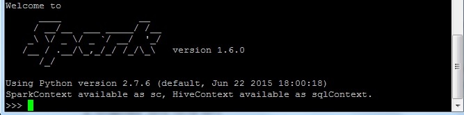
Run pySpark (you can run spark-shell to work in Scala as in the native language): go to the unpacked Spark archive and launch the pyspark in the bin folder (example: spark.apache.org/docs/latest/quick-start.html ). With a successful launch, we get:


It remains to “prepare” our file for SQL queries (in Spark 1.6, for some file types, you can directly make SQL queries without creating a table ). That is, we create a DataFrame (the DataFrame also has a bunch of useful functions ) and from it a table for SQL queries:
1. Download the necessary libraries

>>> from pyspark.sql import SQLContext, Row >>> sqlContext = SQLContext(sc) 

2. Start the text variable as the source file for processing and see what is in the first line:

 >>> text = sc.textFile('  ') >>> text.first() u'2015-09-01\tu' '\t101753' 

In our file lines are separated by tabs. For correct column separation, we use the Map and Split functions using tabs as a separator: map (lambda l: l.split ('\ t')). Select the desired columns from the result of the partition. For this task, we need to know the number of words in a particular search query. Therefore, we take only the query (query column) and the number of words in it (wc column): map (lambda l: Row (query = l [1], wc = len (l [1] .split ('')))).

You can take all the columns of the table in order to make arbitrary SQL queries to it in the future:
map (lambda l: Row (date = l [0], query = l [1], stat = l [2], wc = len (l [1] .split (''))))

Perform these actions in one line

 >>> schema = text.map(lambda l: l.split('\t')).map(lambda l: Row(query=l[1], wc=len(l[1].split(' ')))) 

It remains to convert the schema to a DataFrame, with which you can perform many useful processing operations (examples spark.apache.org/docs/latest/sql-programming-guide.html#dataframe-operations ):

 >>> df = sqlContext.createDataFrame(schema) >>> df.show() +--------------------+---+ | query| wc| +--------------------+---+ | ...| 2| |  | 2| |  | 3| ... 

3. Translate the DataFrame into a table to make SQL queries:

  >>> df.registerTempTable('queryTable') 

4. Create a SQL query for the entire file and upload the result to the output variable:

 >>> output = sqlContext.sql('SELECT wc, COUNT(*) FROM queryTable GROUP BY wc').collect() 

For a 2GB file with 700MB of free RAM, this request took 9 minutes. The progress of the processing process can be seen in the line of the form (... of 53):
INFO TaskSetManager: Finished task 1.0 in stage 8.0 (TID 61) in 11244 ms on localhost (1/53)

We can add additional restrictions:

 >>> outputRealty = sqlContext.sql('SELECT wc, COUNT(*) FROM queryTable WHERE query like "%%" GROUP BY wc').collect() 

It remains to draw a histogram according to this distribution. For example, you can write the output result to the file 'output.txt' and draw the distribution simply in Excel:

 >>> with open('output.txt', 'w') as f: ... f.write('wc \t count \n') ... for line in output: ... f.write(str(line[0]) + '\t' + str(line[1]) + '\n')