Universal Memcomputing Machines as an alternative to Turing Machine

This article can be considered a free translation (although rather an attempt to understand) of this article . And yes, it is written more for mathematicians than for a wide audience.

A small spoiler: in the beginning it seemed to me some kind of magic, but then I understood the catch ...

Nowadays, the Turing machine (hereinafter MT) is the universal definition of the concept of an algorithm, and hence the universal definition of a “problem solver”. There are many other models of the algorithm - lambda calculus, Markov algorithms, etc., but all of them are mathematically equivalent to MT, so even though they are interesting, they do not significantly change anything in the theoretical world.
')
Generally speaking, there are other models - Nondeterministic Turing Machine, Quantum Turing Machines. However, they are (for the time being) only abstract models that cannot be implemented in practice.

Six months ago, an interesting article was published in Science Advances with a computational model that differs significantly from MT and which it is quite possible to put into practice (the article itself was about how they counted the SSP task on real hardware).

And yes. The most interesting thing about this model is that, according to the authors, it is possible to solve (some) tasks from the NP class of complete problems in the time and memory polynomial.

Probably you should immediately stipulate that this result does not mean a solution to the problem. $P = NP$ . After all, the statement of this problem does not “solve the $q \ in NPcomplete$ behind $n ^ {const}$ time ”, and is it possible to simulate a non-deterministic Turing machine on a regular Turing machine in the time polynomial. Since there is a completely different model of calculations, it is impossible to speak about classical classes of complexity.

I myself am skeptical at the moment about the possibility of building this machine in the gland (why I will tell below), but the model itself seemed to me quite interesting for analysis and, quite possibly, it will find application in other areas of science.

Small introduction

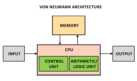
What is a computer (more precisely, the most popular implementation of MT - Arch. Von Neumann) today? Some kind of I / O interface, memory and CPU, which is physically separated from them. In the CPU, there are both the module that controls the progress of the calculations and the blocks that perform these calculations.

The physical separation of the CPU means that we have to spend a lot of time transferring data. Actually for this purpose various levels of cash memory were invented. However, cache memory, of course, makes life easier, but does not solve all data transfer problems.

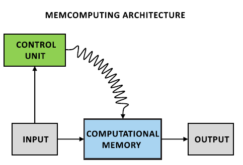
The proposed data model was inspired by the work of the brain (the phrase is rather trite, but it is quite suitable here). Its essence is that the calculations take place not in a separate device, where you need to transfer data, but directly in memory. The order of calculations is controlled by an external device (Control Unit).

This model of computing, called Universal Memcomputing Machines (I did not begin to translate this term. Then I will use the abbreviation UMM).

In this article, we first recall how MT is formally defined, then we will look at the definition of UMM, look at an example of how to set an algorithm for solving a problem on a UMM, consider several properties, including the most important information overhead.

Formal description of the model.

Universal Turing Machine (UTM)

I think you all remember what a Turing machine is (otherwise there is no point in reading this article). Tape, carriage, all things. Let's just remember how it is defined formally.

Turing machine is a tuple

$UTM = (Q, \ Gamma, b, \ Sigma, \ delta, q_0, F),$

Where $Q$ - many possible states,
$\ Gamma$ - many possible ribbon symbols
$b \ in \ Gamma$ - empty character
$\ Sigma$ - many incoming characters
$q_0$ - initial state
$F \ subseteq Q$ - a set of final states

$\ delta: Q \ smallsetminus F \ times \ Gamma \ rightarrow Q \ times \ Gamma \ times \ {L, N, R \}$ where $L, N, R$ accordingly, the shift to the left, without offset, offset to the right. I.e $\ delta$ - our transition table.

Memprocessor

To begin with, let's define our UMM memory cell - memeprocessor.

The memprocessor is defined as a 4-tuple. $(x, y, z, \ sigma)$ where $x$ - the state of the memory processor, $y$ - vector of internal variables. $z$ - vector of "external" variables, that is, variables, connecting different meprocessors. In other words, if $z_1$ and $z_2$ - vectors of external variables of two memprocessors, then two memprocessors are connected $\ Leftrightarrow$ $z_1 \ cap z_2 \ neq \ O$ . Also, if the memprocessor is not connected to anyone, then $z = z (x, y)$ , that is, determined only by the internal state.

And finally $\ sigma [x, y, z] = (x ', y')$ , i.e $\ sigma$ - the operator of the new state.

I want to remind you that the memory processor is not the processor that we usually imagine in our head. It is rather a memory cell that has the function of obtaining a new state (programmable).

Universal Memcomputing Machine (UMM)

Now we introduce the formal definition of UMM. UMM is a model of a computer formed of interconnected meprocessors (which, generally speaking, can be both digital and analog).

$UMM = (M, \ Delta, \ mathcal {P}, S, \ Sigma, p_0, s_0, F),$

Where $M$ - many possible states of the meprocessor
$\ mathcal {P}$ - A set of pointers to the memprocessor (used in $\ delta$ to select the desired memory processors)
$S$ - many indexes $\ alpha$ (number of function used $\ delta$ )
$\ Sigma$ - the initial state of the memprocessor
$p_0$ - initial set of pointers
$s_0$ - initial operator index ($ \ alpha $)
$F \ subseteq M$ - a set of final states

$\ Delta = \ {\ delta _ {\ alpha} \ | \ \ delta _ {\ alpha}: M ^ {m _ {\ alpha}} \ smallsetminus F \ times \ mathcal {P} \ rightarrow M ^ {{m '} _ {\ alpha}} \ times \ mathcal {P} ^ 2 \ times S \},$
Where $m _ {\ alpha} & lt; \ infty$ - the number of memprocessors used as input by the function $\ delta _ {\ alpha}$ , ${m '} _ {\ alpha} & lt; \ infty$ - the number of memory processors used as an exit function $\ delta _ {\ alpha}$ .

By analogy with the Turing machine, as you might have guessed, $\ delta _ {\ alpha}$ - transition functions, an analogue of the state table. If you look at an example, then let $p _ {\ alpha}, {p '} _ {\ alpha}, p _ {\ beta} \ in \ mathcal {P}$ - pointers to memprocessors, $p _ {\ alpha} = \ {i_1, \ dots, i_ {m _ {\ alpha}} \}$ , $x (p)$ - the state vector of these memprocessors, and $\ beta \ in S$ - the index of the next command, then

$\ delta _ {\ alpha} [x (p _ {\ alpha})] = (x '({p'} _ {\ alpha}), \ beta, p _ {\ beta})$

Generally speaking, discarding formalism, the main difference between UMM and MT is that in UMM, affecting a single memory cell (that is, a memory processor), you automatically influence its environment, without additional calls from the Control Unit.

Note 2 properties of the UMM, directly arising from its definition.

Property 1. Intrinsic parallelism (I have not decided how to properly translate this term, so I left it as it is). Any function $\ delta _ {\ alpha}$ can run on any set of processors at the same time. In the Turing machine for this you need to enter additional tapes and heads.
Property 2. Functional polymorphism . It lies in the fact that, unlike the Turing machine, the UMM can have many different operators $\ delta _ {\ alpha}$ .

Generally speaking, it is not so difficult to modify the Turing machine so that it also has these properties, but the authors insist.

And a few more comments on the definition. The UMM, unlike the Turing machine, can have an infinite state space with a finite number of meprocessors (due to the fact that they can be analog).

By the way, UMM can be considered as a generalization of neural networks.

We prove one theorem.

UMM is a universal machine (that is, a machine that can simulate the operation of any MT).

Evidence.

In other words, we need to show that the Turing machine is a special case of the UMM. (whether the opposite is true is not proven, and if the authors of the article are right, then this will be equivalent to proving $P = NP$ )

Let in the definition of UMM, $M = Q \ cup \ Gamma$ . We will designate one of the memory processors as $j_s$ , the rest (possibly infinite qty) as $j$ . Next we define the pointer $p = \ {j_s, j \}$ . $j_s$ we will use as a designation of the state $q \ in Q$ , $j$ as a ribbon symbol ( $\ Gamma$ ).

$\ Delta$ we will consist of a single function $\ delta [x (p)] = (x '(p), p')$ (omit $\ beta$ , since there is only one function). New condition $x '$ determined by the transition table MT, $x '(j_s)$ - there will be a new state, $x '(j)$ - new ribbon symbol. New pointer $p '= \ {j_s, j' \}$ , $j '= j$ if there is no carriage transition, $j '= j + 1$ if we move the carriage to the right, $j '= j - 1$ if left. As a result, when writing to $x$ initial state $q_0$ and the starting character from $\ Sigma$ , with $\ Delta = \ delta$ UTM simulates a universal Turing machine.

The theorem is proved.

Algorithms

Let's look at an example of how to solve problems on the UMM (for now just to get acquainted with the model). Take the subset sum problem ( SSP ) problem.

Let there be many $G \ in \ mathds {Z}$ and given a number $s$ . Is there a subset $K \ subseteq G$ whose sum of elements is equal $s$ .

Exponential algorithm

Let the memprocessors in our UMM be arranged in a matrix form (see the figure). We define three operations.

$\ chi$ - this is directly a calculation. Using activation lines, we can select rows and bounding columns in which calculations are made. The essence of the calculation is in adding the value of the leftmost cell to the entire row.
$\ mu$ - this is a data movement operation. The control node selects two columns and the values from the first are copied to the second. The control node does not necessarily perform the copy operation itself; it simply activates the columns with the necessary lines.
$p$ - operation similar to $\ mu$ , only it takes 1 value and writes it to the column.

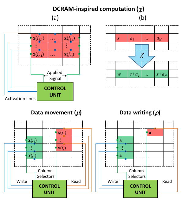
By combining these three operations, we can get the transition function $\ delta = \ mu \ circ \ chi \ circ p$ .

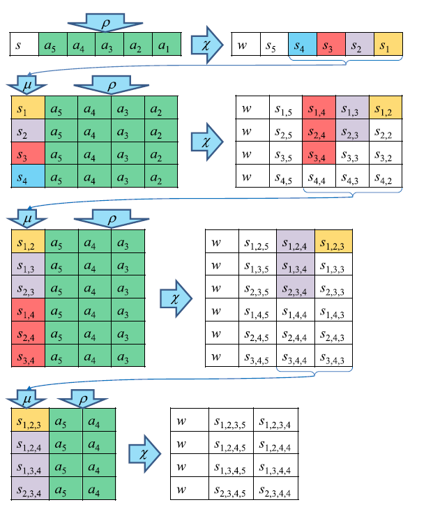
In the first step of the algorithm, we get the sum of all subsets of length $n-1$ on the second step of the subsets $n-2$ and so on. As soon as we found the desired number (it will be in the left column), we found the answer. Each step is performed in one function call. $\ delta$ therefore the algorithm works $n-1$ steps.

Now let's calculate how many processors we need to perform these operations. At iteration k we need $\ binom {n-1} {k-1} (n + 2-k)$ meprotsessorov. Estimation for this expression using Stirling formula - $(n / 2 \ pi) ^ {1/2} 2 ^ {n-1}$ . The number of nodes grows exponentially.

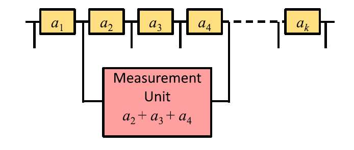
I think now it has become more or less clear what kind of object it is. We now turn to the most delicious that the UMM offers us, namely to the third property - the information overhead .

Exponential Information Overhead

Suppose we have n memprocessors, let us designate the state of the selected memprocessors as $x (p) = (x (j_1), \ dots, x (j_n))$ . The status of a separate memprocessor $x (j) = u_j$ contained in internal variables $u_j \ in M_a$ . $u_j$ - vector. Also for each memprocessor, we divide external variables into 2 groups - “in” and “out” (out of one memprocessor is connected to in another). In the picture the empty circle is a component $(u_j) _h = 0$ . Suppose also that we have a device that, when connected to the desired meprocessor, can be considered at once $u_j$ .

This device, connected to several memprocessors, can consider the state of both, and therefore their global state, defined as $u_ {j_1, j_2} = u_ {j_1} \ diamond u_ {j_2}$ where $\ diamond: R ^ d \ times R ^ d \ rightarrow R ^ d$ - commutative, associative operation, $d = \ dim (u_j)$ . This operation is defined as

$(u_ {j_1} \ diamond u_ {j_2}) _ {h \ star k} = (u_ {j_1}) _ h \ ast (u_ {j_2}) _ k,$

Where $\ star: \ mathds {Z} \ times \ mathds {Z} \ rightarrow \ mathds {Z}$ and $\ ast: R \ times R \ rightarrow R$ - commutative and associative operations with $h \ star 0 = h$ and $x \ ast 0 = 0$ . Moreover, if for $h, k, h ', k'$ performed $h \ star k = h '\ star k'$ then

$(u_ {j_1} \ diamond u_ {j_2}) _ {h \ star k} = (u_ {j_1} \ diamond u_ {j_2}) _ {h \ star k} \ oplus (u_ {j_1} \ diamond u_ { j_2}) _ {h '\ star k'},$

Where $\ oplus: R \ times R \ rightarrow R$ - commutative, associative operation, for which $x \ oplus 0 = x$ .

Now having a lot $G = \ {a_1, \ dots, a_n \}$ integers, we define the message $m = (a _ {\ sigma_1} \ star \ dots \ star a _ {\ sigma_k}) \ cup (a _ {\ sigma_1}, \ dots, a _ {\ sigma_k})$ where $(\ sigma_1, \ dots, \ sigma_k)$ - indexes taken from various subsets $\ {1, \ dots, n \}$ . Thus many messages $M$ consists of $\ sum_ {j = 0} ^ m \ binom {n} {j} = 2 ^ n$ equally likely messages $m$ The amount of information on Shannon is equal to $I (m) = - \ log_2 (2 ^ {- n}) = n$

Now, taking n memprocessors, we expose nonzero components $u_ {j_0}, u_ {j_h}$ where $h \ in \ {1, \ dots, n \}$ . So we coded all the elements. $G$ on the memory processors. On the other hand, by connecting to the necessary meprocessors and reading their global state (according to the formulas, the sum of the elements is obtained there), we can consider any possible state m. In other words, n memprocessors can encode (compress information if you wish) about $2 ^ n$ messages at the same time.

SSP solution algorithm using Exponential Information Overhead

Here I have to say that I could not understand the details of this algorithm (it turned out that I am not so good at electrical engineering and signal processing, and the authors apparently decided not to paint everything for such ignoramuses), but the general idea is .

For starters, they offer a look at the function

$g (x) = -1 + \ prod_ {j = 1} ^ n (1 + e ^ {i 2 \ pi a_j x})$

If we open the brackets, then we will have works on various sets of indices $j$ (denote such a set as $P$ ), and they are equal

$\ prod_ {j \ in P} e ^ {i 2 \ pi a_j x} = \ exp \ left (i 2 \ pi x \ sum_ {j \ in P} a_j \ right)$

In other words, our function $g$ contains information about the sums of all subsets $G$ . Now, if we consider the function g as a signal source, then each exponent contributes to the resulting signal, with the contribution with frequency $\ sum_ {j \ in P} a_j$ .

Now, all we need is to apply a Fourier transform to this signal and see what frequencies we have in the signal. If we have a component with a frequency $s$ then the subset $G$ with sum $s$ exists.

If we solve this problem on a regular computer, now we could apply a fast Fourier transform. Let us estimate the asymptotics.

To do this, we estimate the number of points that need to be taken from the signal. By the Kotelnikov theorem, these points need $N = 2 f_ {max} + 1$ where $f_ {max} & lt; n \ max \ {| a_j | \}$ - Evaluation of the maximum possible value of frequency. In the article, the authors introduced an additional variable. $p$ which is proportional $N$ and considered the asymptotics through it.

Thus, using FFT we can solve the problem for $O (p \ log (p))$ . Here it should be noted that, as in the backpack problem (and SSP is a special case of the backpack problem), $ p $ grows exponentially. For our problem, you can also use the Görtsel algorithm, which will give us $O (n p)$ . The proposed method allows the authors to get rid of $p$ asymptotic, which will give us linear time.

Now, in your own words (for more detailed consideration, refer to the original articles), how they achieved this.

Take $n$ analog memory processors, the internal value of which will be the value of a certain number of $G$ . As operators $\ star$ and $\ ast$ taken, respectively, addition and multiplication.

But it is in our model. In iron, it turns out that each memprocessor is a signal generator with its own frequency (corresponding to the number of $G$ ), the general state of the memory processors is simply the addition of a signal. It turns out that these memory processors simulate the function $g$ .

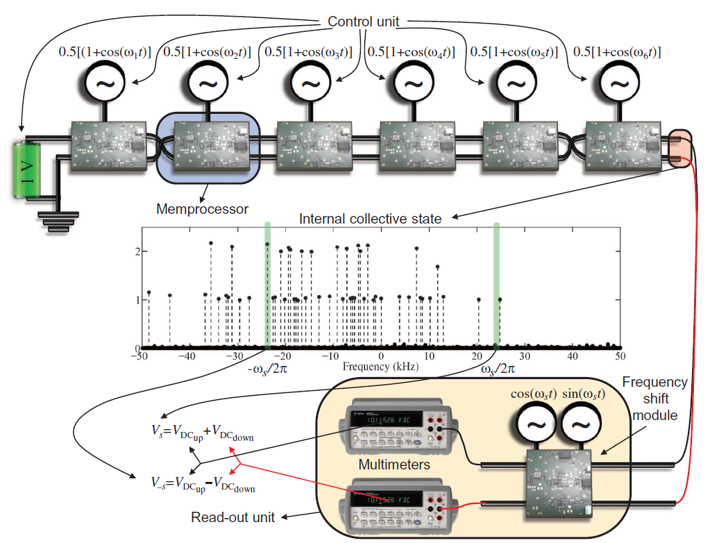
Well, now, in order to read the result, you need to check if there is a given frequency in the signal. Instead of implementing FFT, they made a piece of hardware that only skips a given frequency (I didn’t quite understand how, but my knowledge in electronics is to blame), which is already working for a constant time.

Total time asymptotics in general amounted to $O (1)$ , asymptotics for the memprocessor was $O (n)$ . Let us fireworks? Do not hurry.

Some problems of the model

In fact, the authors slyly shifted the “complicated” part of the task, which gives us the exhibitor, from the program part to the technical part. In an earlier article about this in general, not a word, in July they admit it, but only a few lines.

It's all about signal coding (I found a clear explanation here ). Due to the fact that we encode analog signals, and use discrete signal generators, we now need exponential accuracy in determining the signal level (in the piece of hardware that isolates the desired frequency), which may require the time exponent.

The authors argue that this trouble can be circumvented, if instead of discrete signal generators use analog. But I have big doubts that you can use analog circuits for any $n$ and at the same time not to drown in the noise (because of them at the time they abandoned analog computers and began to use digital).

Total

Wonderful magic did not happen. NP full problems are still difficult to calculate. So why did I write all this? Mainly because at least the physical implementation is complex, the model itself seems very interesting to me, and their study is necessary. Soon (if not now), such models will be of great importance in many areas of science.

For example, as I mentioned, neural networks are a special case of UMM. It is possible that we will learn a little more about neural networks if we look at them from the other side using a slightly different mate. apparatus.

Source: https://habr.com/ru/post/274593/

All Articles