Fourier transform boundedness or why you should trust your hearing
For the last several decades, the task of recognizing chords in a musical composition was set quite often. It would seem that this not so original service was and remains quite common among applications that work with sound (Ableton, Guitar Pro), however, a universal algorithm that always works does not exist until now. In this article I will try to reveal one of the many reasons for the imperfect operation of such services using the example of algorithms based on the Fourier transform.
Most audio formats store information in the form of amplitude versus time (for example, .wav) or in the form of frequency conversion coefficients (.mp3, .aac, .ogg), but modern sophisticated digital signal processing algorithms work with the frequency component of sounds. We have to deal with a double transition, from the amplitude to the frequency domain, then back. At the moment, the implementation of such a transition without loss in quality is a fairly common problem with many ambiguous solutions.
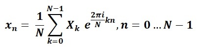
To decompose the signal into frequencies, the Fourier transform, which is widespread in many areas, is used. Since most digital signal processing algorithms have to deal with some sampling of the signal amplitude at a specific point in time, it is convenient to use one of the many modifications of the Fourier transform — the discrete Fourier transform. In its classical interpretation, the Fourier transform is a sum of the form:

')
where N is the number of components of the decomposition,
xn, n = 0 ... N - 1 - the value of the reference signal at time n,
Xk, k = 0 ... N - 1 - output values of the transformation, which are the desired frequency values,
k - frequency index.
The values of Xk obtained as a result of direct transformation represent a set of complex values — Re (Xk) + i * Im (Xk) pairs, which characterize the amplitude and the initial phase of the harmonic signal. Applying the inverse Fourier transform to the values obtained
we will restore the original signal with some accuracy. In practice, it is often necessary to work with large amounts of data. To significantly speed up the computation, the Fast Fourier Transform is used, called the FFT (Fast Fourier Transform) in many modern libraries. FFT also works with complex numbers and is different in that the size of the transformation itself is necessarily a power of two, in practice we most often see the numbers 1024 or 2048. We vary the size of the transformation and the sample size, we get a set of samples close to the real signal, we act on it the inverse Fourier transform, and at the output in front of us are the original frequencies, which means that getting the chord sequence played should not be particularly difficult.
But. Fourier transform of any kind is a complex universal tool, strongly dependent on the data supplied to it. The continuous Fourier transform is a development of the idea of Fourier series, more generalized, the resulting frequency values of which are complex numbers. We look at the classic direct transform.
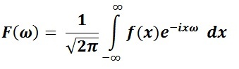
and we see in its implementation an integral on an infinite interval, on a discrete transformation - this is an infinite sum of a series. And we can only speak about the fairness of the equality of the right and left parts when the original function is a function of infinite length, only when we have an infinite signal before us. It is easy to agree that in practice such signals are not often met.
Create an artificial signal corresponding to the note A, taken in two different octaves (frequencies equal to 440 Hz and 3440 Hz, respectively), let us pass it through the direct Fourier transform, and then through the opposite:
Run the Scilab code and see that the original signal ( x ) and the signal obtained by the inverse transform ( z1 ), to put it mildly, are different:

Fig.1 Graph of the function x of the original signal (red color) and the restored signal z1 (yellow color)
How to avoid such restrictions with infinity? Since the transfer of the signal to the frequency representation using FFT is performed only by blocks, for each such block we can increase the sampling frequency, thereby increasing the size of the FFT block and, accordingly, the number of transform coefficients. This will give us a more accurate frequency result per unit of time. Reasonable enough approach.
But no matter how much we approach the length of the gap to infinity, inaccuracies will still occur. The FFT does not know anything about the original harmonics of the function. In our case, there was a frequency of 440 Hz, and the FFT turned it into a set of harmonics with distorted frequencies, although close in meaning to the original one. Therefore, the obtained signal values are only close to the original. To eliminate this distortion, the so-called window functions are used. Before decomposition, the FFT block is multiplied by the window function W (ω - t) , where t is the instant of time corresponding to the current count. The main influence of the window function is to reduce the coefficients in front of the imaginary frequencies in the decomposition, thereby reducing their contribution to the final frequency pattern.
But how will we understand that we have cut off the truly “minor” frequency peaks? Of course, you can try to experiment with partitions and their length, the length of the intervals with zero coefficients outside the window function, but this will only partially smooth out the final picture. To take at least the case when the sought-for notes have rather low frequencies, here we can get imaginary frequencies that are much higher than the original material!
Here it is obviously worth trying experiments with window functions of a different type. For example, the classic rectangular window function
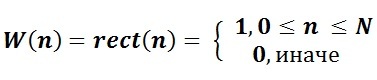
will keep all the original frequencies. But if we take, say, a triangular window

it will become obvious that the marginal outliers will simply be cut off, with the highest probability there will be the most pure information.
But. Again, we generate a simple bounded signal and calculate its spectrum:
Source signal x:
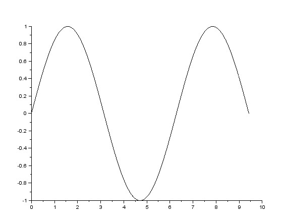
Fig.2 Source signal x
Fig.3. Spectrum of signal y
What do we see? The spectrum has ceased to be limited, unnecessary values have been formed on both its sides, moreover, their infinite number! What happened? At those two points where contact with the edges of the window function occurred, the function is no longer smooth. At the input, the Fourier transform expects to see a signal representing the sum of simple sinusoids, where the points of discontinuity can only be obtained using an infinite sum of these sinusoids.
Here we are directly confronted with the most genuine uncertainty principle for the field of signal processing. The principle here is called the Benedick Theorem: a function cannot be simultaneously limited in the range of time and in the range of frequency. In a more rigorous formulation, the theorem is: function in space and its mapping Fourier
  cannot have the same support function at the same time on coverages with a Lebesgue measure. And if you rarely have to deal with signals of infinite length, and this area for practice is of lesser importance, then what about the case when the signal has a finite length?
And here we can not do without the most well-known theorem in the theory of sound signal processing - the Kotelnikov-Naykwaist-Shannon theorem, which in one of its interpretations reads as follows: any analog signal can be reconstructed with any accuracy according to its discrete readings when the values its samples are f> 2Fmax, where Fmax is the maximum frequency to which the spectrum of the original signal is limited. Based on this theorem and the Benedik theorem, we conclude that at the moment there are no real signals that can be presented with infinitely high accuracy in a discrete and limited form . We will always either deal with a signal of infinitely long length, or we will receive in a limited signal inaccuracies of varying degrees, which in the end can significantly spoil the picture of the original audio recording.
Of course, the developers of such services, working with sounds, solve this problem to some extent. Use step interpolation, different types of linear interpolation, low-pass filters to deal with samples exceeding half the sampling rate. Their most common drawbacks are the data that are only roughly approximated to the original frequencies, as well as the presence of high-frequency garbage. However, the audio recordings with which we have to deal are also far from ideal. High noise, recording speed, sound quality. Here you need to be able to adapt to each signal, calculate the speed of the game, the duration of the chords, extinguish the white (at best) noise, but this is a completely different story.
Most audio formats store information in the form of amplitude versus time (for example, .wav) or in the form of frequency conversion coefficients (.mp3, .aac, .ogg), but modern sophisticated digital signal processing algorithms work with the frequency component of sounds. We have to deal with a double transition, from the amplitude to the frequency domain, then back. At the moment, the implementation of such a transition without loss in quality is a fairly common problem with many ambiguous solutions.
To decompose the signal into frequencies, the Fourier transform, which is widespread in many areas, is used. Since most digital signal processing algorithms have to deal with some sampling of the signal amplitude at a specific point in time, it is convenient to use one of the many modifications of the Fourier transform — the discrete Fourier transform. In its classical interpretation, the Fourier transform is a sum of the form:
')
where N is the number of components of the decomposition,
xn, n = 0 ... N - 1 - the value of the reference signal at time n,
Xk, k = 0 ... N - 1 - output values of the transformation, which are the desired frequency values,
k - frequency index.
The values of Xk obtained as a result of direct transformation represent a set of complex values — Re (Xk) + i * Im (Xk) pairs, which characterize the amplitude and the initial phase of the harmonic signal. Applying the inverse Fourier transform to the values obtained
we will restore the original signal with some accuracy. In practice, it is often necessary to work with large amounts of data. To significantly speed up the computation, the Fast Fourier Transform is used, called the FFT (Fast Fourier Transform) in many modern libraries. FFT also works with complex numbers and is different in that the size of the transformation itself is necessarily a power of two, in practice we most often see the numbers 1024 or 2048. We vary the size of the transformation and the sample size, we get a set of samples close to the real signal, we act on it the inverse Fourier transform, and at the output in front of us are the original frequencies, which means that getting the chord sequence played should not be particularly difficult.
But. Fourier transform of any kind is a complex universal tool, strongly dependent on the data supplied to it. The continuous Fourier transform is a development of the idea of Fourier series, more generalized, the resulting frequency values of which are complex numbers. We look at the classic direct transform.
and we see in its implementation an integral on an infinite interval, on a discrete transformation - this is an infinite sum of a series. And we can only speak about the fairness of the equality of the right and left parts when the original function is a function of infinite length, only when we have an infinite signal before us. It is easy to agree that in practice such signals are not often met.
Create an artificial signal corresponding to the note A, taken in two different octaves (frequencies equal to 440 Hz and 3440 Hz, respectively), let us pass it through the direct Fourier transform, and then through the opposite:
dt = 0.001; T = 1; t=0:dt:T; w = 440; q = 2^(1/12); // x = cos(2*%pi*w*t*q^1) + cos(2*%pi*w*t*q^4); scf(0); plot2d(x, rect=[0,0,1200,2]); // y = fft(x); scf(1); plot(y); // z = fft(y,-1); z1 = z/(T/dt); scf(2); plot2d(x, style=[color("red")], rect=[0,0,1200,2]); plot2d(z1,style=[color("green")], rect=[0,0,1200,2]); Run the Scilab code and see that the original signal ( x ) and the signal obtained by the inverse transform ( z1 ), to put it mildly, are different:
Fig.1 Graph of the function x of the original signal (red color) and the restored signal z1 (yellow color)
How to avoid such restrictions with infinity? Since the transfer of the signal to the frequency representation using FFT is performed only by blocks, for each such block we can increase the sampling frequency, thereby increasing the size of the FFT block and, accordingly, the number of transform coefficients. This will give us a more accurate frequency result per unit of time. Reasonable enough approach.
But no matter how much we approach the length of the gap to infinity, inaccuracies will still occur. The FFT does not know anything about the original harmonics of the function. In our case, there was a frequency of 440 Hz, and the FFT turned it into a set of harmonics with distorted frequencies, although close in meaning to the original one. Therefore, the obtained signal values are only close to the original. To eliminate this distortion, the so-called window functions are used. Before decomposition, the FFT block is multiplied by the window function W (ω - t) , where t is the instant of time corresponding to the current count. The main influence of the window function is to reduce the coefficients in front of the imaginary frequencies in the decomposition, thereby reducing their contribution to the final frequency pattern.
But how will we understand that we have cut off the truly “minor” frequency peaks? Of course, you can try to experiment with partitions and their length, the length of the intervals with zero coefficients outside the window function, but this will only partially smooth out the final picture. To take at least the case when the sought-for notes have rather low frequencies, here we can get imaginary frequencies that are much higher than the original material!
Here it is obviously worth trying experiments with window functions of a different type. For example, the classic rectangular window function
will keep all the original frequencies. But if we take, say, a triangular window
it will become obvious that the marginal outliers will simply be cut off, with the highest probability there will be the most pure information.
But. Again, we generate a simple bounded signal and calculate its spectrum:
scf(0); t=0:0.0001:3*%pi; x = sin(t); plot2d(t,x); y = simp(fft(x)); scf(1); plot2d(y, rect = [-100, -10000, 40000, 10000]); disp(y(1000)); Source signal x:
Fig.2 Source signal x
Fig.3. Spectrum of signal y
What do we see? The spectrum has ceased to be limited, unnecessary values have been formed on both its sides, moreover, their infinite number! What happened? At those two points where contact with the edges of the window function occurred, the function is no longer smooth. At the input, the Fourier transform expects to see a signal representing the sum of simple sinusoids, where the points of discontinuity can only be obtained using an infinite sum of these sinusoids.
Here we are directly confronted with the most genuine uncertainty principle for the field of signal processing. The principle here is called the Benedick Theorem: a function cannot be simultaneously limited in the range of time and in the range of frequency. In a more rigorous formulation, the theorem is: function in space
and its mapping Fourier cannot have the same support function at the same time on coverages with a Lebesgue measure. And if you rarely have to deal with signals of infinite length, and this area for practice is of lesser importance, then what about the case when the signal has a finite length?And here we can not do without the most well-known theorem in the theory of sound signal processing - the Kotelnikov-Naykwaist-Shannon theorem, which in one of its interpretations reads as follows: any analog signal can be reconstructed with any accuracy according to its discrete readings when the values its samples are f> 2Fmax, where Fmax is the maximum frequency to which the spectrum of the original signal is limited. Based on this theorem and the Benedik theorem, we conclude that at the moment there are no real signals that can be presented with infinitely high accuracy in a discrete and limited form . We will always either deal with a signal of infinitely long length, or we will receive in a limited signal inaccuracies of varying degrees, which in the end can significantly spoil the picture of the original audio recording.
Of course, the developers of such services, working with sounds, solve this problem to some extent. Use step interpolation, different types of linear interpolation, low-pass filters to deal with samples exceeding half the sampling rate. Their most common drawbacks are the data that are only roughly approximated to the original frequencies, as well as the presence of high-frequency garbage. However, the audio recordings with which we have to deal are also far from ideal. High noise, recording speed, sound quality. Here you need to be able to adapt to each signal, calculate the speed of the game, the duration of the chords, extinguish the white (at best) noise, but this is a completely different story.
Source: https://habr.com/ru/post/274175/
All Articles