Kaggle and Titanic - another solution using Python
I want to share my experience with the task of the famous Kaggle machine learning competition. This competition is positioned as a competition for beginners, and I just had almost no practical experience in this area. I knew a bit of theory, but I almost didn’t deal with real data and did not work closely with python. In the end, after spending a couple of New Year's Eve evenings, I scored 0.80383 (the first quarter of the rating).

')
We include suitable for the work of music and begin the study.
The contest "on the Titanic" has already been repeatedly noted on Habré. I would especially like to mention the latest article from the list - it turns out that researching data can be no less intriguing than a good detective novel, and an excellent result (0.81340) can be obtained not only by the Random Forest classifier.
I would also like to note an article about another competition. From it you can understand exactly how the brain of the researcher should work and that most of the time should be devoted to preliminary analysis and data processing.
To solve the problem, I use the Python-technology stack. This approach is not the only possible one: there are R, Matlab, Mathematica, Azure Machine Learning, Apache Weka, Java-ML and I think the list can be continued for a long time. Using Python has a number of advantages: there are really a lot of libraries and they are of excellent quality, and since most of them are wrappers over C-code, they are also quite fast. In addition, the constructed model can be easily put into operation.
I must admit that I am not a very big fan of scripting non-strictly typed languages, but the wealth of libraries for python does not allow it to be ignored in any way.
We will run everything under Linux (Ubuntu 14.04). You need: python 2.7, seaborn, matplotlib, sklearn, xgboost, pandas. In general, only pandas and sklearn are required, and the rest are needed for illustration.
Under Linux, libraries for Python can be installed in two ways: by the regular package manager (deb) manager or via the Python utility pip.
Installing deb packages is easier and faster, but often the libraries are outdated there (stability is above all).
Installing packages via pip is longer (it will be compiled), but with it you can count on getting fresh versions of packages.
So how is it better to install packages? I use a compromise: I put massive and requiring multiple dependencies to build NumPy and SciPy from DEB-packages.
And the rest, lighter packages, install via pip.
If I have forgotten something, then all the necessary packages are usually easily calculated and installed in a similar way.
Users of other platforms need to take similar steps to install packages. But there is a much simpler option: there are already precompiled distributions with python and almost all the necessary libraries. I have not tried them myself, but at first glance they look promising.
Download the source data for the problem and see what we were given.
Frankly speaking, we don’t have a lot of data - only 891 passengers in the train-sample, and 418 in the test-sample (one line goes to the header with a list of fields).
Open train.csv in any tabular processor (I use LibreOffice Calc) to visually see the data.
We see the following:
It seems about everything is clear, we go directly to working with data.
In order not to make noise, the next code will immediately cite all used imports:
Probably most of my motivation for writing this article is caused by the enthusiasm from working with the pandas package. I knew about the existence of this technology, but I could not even imagine how pleasant it was to work with it. Pandas is Excel on the command line with convenient I / O functionality and tabular data processing.
Load both selections.
We collect both samples (train-sample and test-sample) into one total all-sample.
Why do this, because in the test sample there is no field with a resulting survival flag? The complete sample is useful for calculating statistics for all other fields (averages, medians, quantiles, minima and maxima), as well as the relationships between these fields. That is, considering statistics only for train-sampling, we actually ignore some very useful information for us.
Data analysis in Python can be done in several ways at once, for example:
We will try all three, but first we will launch the simplest text version. We derive survival statistics depending on the class and gender.
We see that women were first planted into the boats first — the woman’s survival rate is 96.8%, 92.1% and 50% depending on the class of the ticket. The chance of a man’s survival is much lower and amounts to 36.9%, 15.7% and 13.5% respectively.
With the help of pandas, we quickly calculate a summary of all the numerical fields of both samples - separately for men and for women.
It is seen that in the middle and percentiles everything is completely flat. But for men, samples differ in maximums by age and by ticket price. Women in both samples also have a difference in the maximum age.
Let's collect a small digest for the full sample - it will be needed for the further conversion of the samples. In particular, we need the values that will be substituted for the missing ones, as well as various reference books for translating text values into numeric values. The fact is that many classifiers can work only with numbers, so somehow we have to translate categorical attributes into numeric ones, but regardless of the way of conversion, we will need reference books of these values.
A little explanation of the digest fields:
We build reference books for recovering missing data (medians) using a combined sample. But reference books for the translation of categorical signs - only for test data. The idea was the following: let's say we have the last name “Ivanov” in the train-set, but there is no this name in the test-set. The knowledge inside the classifier that “Ivanov” survived (or did not survive) does not help in the evaluation of the test set, since this name still does not exist in the test set. Therefore, in the directory add only those names that are in the test-set. An even more correct way would be to add only the intersection of signs to the directory (only those signs that are in both sets) - I tried, but the verification result deteriorated by 3 percent.
Now we need to highlight the signs. As already mentioned, many classifiers can only work with numbers, so we need:
There are two ways to convert a categorical feature into a numeric one. We can consider the problem on the example of the passenger floor.
In the first version, we simply change the floor to a certain number, for example, we can replace female with 0, and male with 1 ( roundwheel and wand - very convenient to remember ). This option does not increase the number of signs, however, the “more” and “less” relation now appears inside the sign for its values. In the case when there are many values, such an unexpected property of the feature is not always desirable and can lead to problems in geometric classifiers.
The second conversion option is to have two columns, “sex_male” and “sex_female”. In the case of a male, we will assign sex_male = 1, sex_female = 0. In the case of the female, vice versa: sex_male = 0, sex_female = 1. We now avoid “more” / “less” relations, but now we have more signs, and the more signs, the more data we need to train the classifier — this problem is known as the “curse of dimensionality” . Especially difficult is the situation when there are a lot of attribute values, for example ticket IDs, in such cases, for example, you can fold back rarely occurring values by substituting some special tag instead of them - thus reducing the total number of attributes after the extension.
A small spoiler: we bet first on the Random Forest classifier. Firstly, everyone does this , and secondly, it does not require expansion of features, is resistant to the scale of feature values and is calculated quickly. Despite this, we are preparing the signs in a general universal form, since the main goal set before us is to explore the principles of working with sklearn and possibilities.
Thus, we replace some categorical signs with numbers, some expand, some and replace and expand. We do not save on the number of signs, because in the future we can always choose which ones will be involved in the work.
In most manuals and examples from the network, the original data sets are very freely modified: the original columns are replaced with new values, unnecessary columns are deleted, etc. There is no need for this as long as we have a sufficient amount of RAM: it is always better to add new features to the set without altering the existing data, since later pandas will always allow us to select only the ones we need.
Create a method for converting datasets.
A small explanation of the addition of new features:
In general, we add to the signs in general everything that comes to mind. It can be seen that some signs duplicate each other (for example, expansion and replacement of gender), some clearly correlate with each other (ticket class and ticket price), some are clearly meaningless (the port of landing is unlikely to affect survival). We will deal with all this later - when we make the selection of signs for training.
Let's transform both available sets and also create a combined set again.
Although we are aiming at using Random Forest, I want to try other classifiers. And with them there is the following problem: many classifiers are sensitive to the scale of features. In other words, if we have one attribute with values from [–10.5] and a second characteristic with values [0, 0,000], then the same percentage error on both signs will lead to a large difference in absolute value and the classifier will interpret the second characteristic as more important.
To avoid this, we reduce all numeric (and we no longer have any other) signs to the same scale [-1,1] and zero mean value. To do this in sklearn can be very simple.
First, we calculate the scaling factors (the complete set again came in handy), and then we scale both sets individually.
Well, the moment has come when we can select those signs with which we will work further.
Just put a comment on unnecessary and start training. What exactly is not needed - you decide .
Since now we have a column in which the range is recorded in which the age of the passenger falls, we estimate the survival rate depending on the age (range).
We see that the chances of survival are great for children under 5 years old, and already in old age the chance to survive decreases with age. But this does not apply to women - a woman has a great chance of survival at any age.
Let's try visualization from seaborn - it gives very beautiful pictures, although I am more used to the text.

Beautiful, but for example the correlation in a pair of "class-floor" is not very clear.
Let us evaluate the importance of our features using the SelectKBest algorithm.
Here you have an article describing exactly how he does it. Other strategies can be specified in the SelectKBest parameters.
In principle, we already know everything - gender is very important. Titles are important - but they have a strong correlation with sex. The ticket class is important and in some way the F deck.
Before starting any classification, we need to understand how we will evaluate it. In the case of Kaggle contests, everything is very simple: we just read their rules. In the case of the Titanic, the estimate will be the ratio of the correct classifier ratings to the total number of passengers. In other words, this estimate is called accuracy .
But before sending the classification result for the test sample to an assessment in Kaggle, we would be nice to first understand for ourselves at least the approximate quality of our classifier. To understand this, we can only use train-sampling, since only it contains labeled data. But the question remains - how exactly?
Often in examples you can see something like this:
That is, we train the classifier on the train-set, after which we check it on it. Undoubtedly, to some extent, this gives a certain assessment of the quality of the classifier’s work, but in general this approach is incorrect. The classifier should not describe the data on which he was trained, but some model that generated this data. Otherwise, the classifier perfectly adapts to the train-sample, when checking it shows excellent results, but when checking on some other data set it merges with a bang. What is called overfitting .
The correct approach would be to divide the available train-set into a number of pieces. We can take a few of them, train the classifier on them, and then check his work for the rest. You can produce this process several times just by shuffling the pieces. In sklearn, this process is called cross-validation .
You can already imagine in your head the cycles that will share data, produce training and assessment, but the trick is that all you need to implement this in sklearn is to determine a strategy.
Here we define a rather complicated process: the training data will be divided into three pieces, and the records will fall into each piece in a random way (to level the possible dependence on the order), besides the strategy will track the ratio of classes in each piece to be approximately equal. Thus, we will perform three measurements on pieces 1 + 2 vs 3, 1 + 3 vs 2, 2 + 3 vs 1 - after that we will be able to get an average assessment of the accuracy of the classifier (which will characterize the quality of work), as well as the variance of the assessment (which will be characterize the stability of his work).
Now let's test the work of various classifiers.
KNeighborsClassifier :
SGDClassifier :
SVC :
GaussianNB :
LinearRegression :
The linear_scorer method is needed because LinearRegression is a regression that returns any real number. Accordingly, we divide the scale by the border of 0.5 and reduce any numbers to two classes - 0 and 1.
LogisticRegression :
RandomForestClassifier :
Random Forest won the algorithm and its dispersion is not bad - it seems it is stable.
Everything seems to be good and you can send the result, but there is only one muddy moment left: each classifier has its own parameters - how can we understand that we have chosen the best option? Without a doubt, you can sit for a long time and sort through the parameters manually - but what if you entrust this work to a computer?
Selection can be made even thinner if there is time and desire - either by changing the parameters, or using a different selection strategy, for example, RandomizedSearchCV .
Everyone praises xgboost - let's try it too.
For some reason, the training hung when using all the cores, so I limited myself to one thread (n_jobs = 1), but in single-threaded mode, training and classification in xgboost works very quickly.
The classifier is selected, the parameters are calculated - it remains to generate the result and send it to Kaggle for review.
In general, it is worth noting a few points in such competitions, which seemed interesting to me:
Looking through the top contestants, it is impossible not to notice the people who scored 1 (all the answers are correct) - and some got it from the very first attempt.
The next option comes to mind: someone registered an account with which he began to select (no more than 10 attempts per day are allowed) the correct answers. If I understand correctly, this is a kind of weighing task .
However, after thinking a little more, it is impossible not to smile at our guess: we are talking about a task, the answers for which have long been known! In fact, the death of Titanic was a shock to his contemporaries, and films, books and documentaries were devoted to this event. And most likely somewhere there is a complete list of names of passengers of the Titanic with a description of their fate. But this is no longer true for machine learning.
However, from this it is possible and necessary to draw a conclusion that I am going to apply in the following competitions - not necessarily (if this is not prohibited by the rules of the competition) to be limited only to the data that the organizer issued. For example, by a certain time and place, weather conditions, the state of securities markets, exchange rates, whether the day is a holiday can be identified - in other words, you can marry data from the organizers with any available public data sets that can help in describing the characteristics of the model.
The full script code is here . Do not forget to choose the signs for training.
')
Titanic
We include suitable for the work of music and begin the study.
The contest "on the Titanic" has already been repeatedly noted on Habré. I would especially like to mention the latest article from the list - it turns out that researching data can be no less intriguing than a good detective novel, and an excellent result (0.81340) can be obtained not only by the Random Forest classifier.
- habrahabr.ru/company/microsoft/blog/268039 - Predicting the survival of passengers of the Titanic using Azure Machine Learning
- habrahabr.ru/post/165001 - Data Mining: Primary data processing using DBMS
- habrahabr.ru/company/mlclass/blog/248779 - When there is really a lot of data: Vowpal Wabbit
- habrahabr.ru/post/272201 - The steady beauty of indecent models
- habrahabr.ru/post/202090 - Basics of data analysis in python using pandas + sklearn
- habrahabr.ru/company/mlclass/blog/270973 - Titanic on Kaggle: you do not finish reading this post to the end
I would also like to note an article about another competition. From it you can understand exactly how the brain of the researcher should work and that most of the time should be devoted to preliminary analysis and data processing.
- habrahabr.ru/post/270367 - How I won the competition BigData from Beeline
Tools
To solve the problem, I use the Python-technology stack. This approach is not the only possible one: there are R, Matlab, Mathematica, Azure Machine Learning, Apache Weka, Java-ML and I think the list can be continued for a long time. Using Python has a number of advantages: there are really a lot of libraries and they are of excellent quality, and since most of them are wrappers over C-code, they are also quite fast. In addition, the constructed model can be easily put into operation.
I must admit that I am not a very big fan of scripting non-strictly typed languages, but the wealth of libraries for python does not allow it to be ignored in any way.
We will run everything under Linux (Ubuntu 14.04). You need: python 2.7, seaborn, matplotlib, sklearn, xgboost, pandas. In general, only pandas and sklearn are required, and the rest are needed for illustration.
Under Linux, libraries for Python can be installed in two ways: by the regular package manager (deb) manager or via the Python utility pip.
Installing deb packages is easier and faster, but often the libraries are outdated there (stability is above all).
# /usr/lib/python2.7/dist-packages/ $ sudo apt-get install python-matplotlib Installing packages via pip is longer (it will be compiled), but with it you can count on getting fresh versions of packages.
# /usr/local/lib/python2.7/dist-packages/ $ sudo pip install matplotlib So how is it better to install packages? I use a compromise: I put massive and requiring multiple dependencies to build NumPy and SciPy from DEB-packages.
$ sudo apt-get install python $ sudo apt-get install python-pip $ sudo apt-get install python-numpy $ sudo apt-get install python-scipy $ sudo apt-get install ipython And the rest, lighter packages, install via pip.
$ sudo pip install pandas $ sudo pip install matplotlib==1.4.3 $ sudo pip install skimage $ sudo pip install sklearn $ sudo pip install seaborn $ sudo pip install statsmodels $ sudo pip install xgboost If I have forgotten something, then all the necessary packages are usually easily calculated and installed in a similar way.
Users of other platforms need to take similar steps to install packages. But there is a much simpler option: there are already precompiled distributions with python and almost all the necessary libraries. I have not tried them myself, but at first glance they look promising.
- www.continuum.io/downloads - Anaconda
- www.enthought.com/products/canopy - Canopy
Data
Download the source data for the problem and see what we were given.
$ wc -l train.csv test.csv 892 train.csv 419 test.csv 1311 total Frankly speaking, we don’t have a lot of data - only 891 passengers in the train-sample, and 418 in the test-sample (one line goes to the header with a list of fields).
Open train.csv in any tabular processor (I use LibreOffice Calc) to visually see the data.
$ libreoffice --calc train.csv We see the following:
- Not everyone's age is filled
- Tickets have a strange and inconsistent format.
- Names have a title (miss, mr, mrs, etc.)
- There are very few people who have cabin numbers ( there is a chilling story about why)
- In the existing rooms of the cabins, the deck code is apparently registered (as it turned out )
- Also, according to the article , the side is encrypted in the cabin room.
- Sort by name. It is evident that many traveled in families, and the scale of the tragedy is visible - often the families were separated, only a part survived.
- Sort by ticket. It can be seen that several people traveled along the same ticket code at once, often with different surnames. A quick glance seems to show that people with the same ticket number often share the same fate.
- Some passengers do not have a landing port
It seems about everything is clear, we go directly to working with data.
Data loading
In order not to make noise, the next code will immediately cite all used imports:
Script header
# coding = utf8
import pandas as pd
import numpy as np
import matplotlib.pyplot as plt
import xgboost as xgb
import re
import seaborn as sns
from sklearn.linear_model import LinearRegression
from sklearn.linear_model import LogisticRegression
from sklearn.linear_model import SGDClassifier
from sklearn.ensemble import RandomForestClassifier
from sklearn.grid_search import GridSearchCV
from sklearn.neighbors import KNeighborsClassifier
from sklearn.naive_bayes import GaussianNB
from sklearn.svm import SVC
from sklearn.feature_selection import SelectKBest, f_classif
from sklearn.cross_validation import StratifiedKFold
from sklearn.cross_validation import KFold
from sklearn.cross_validation import cross_val_score
from sklearn.preprocessing import StandardScaler
from sklearn import metrics
pd.set_option ('display.width', 256)
Probably most of my motivation for writing this article is caused by the enthusiasm from working with the pandas package. I knew about the existence of this technology, but I could not even imagine how pleasant it was to work with it. Pandas is Excel on the command line with convenient I / O functionality and tabular data processing.
Load both selections.
train_data = pd.read_csv("data/train.csv") test_data = pd.read_csv("data/test.csv") We collect both samples (train-sample and test-sample) into one total all-sample.
all_data = pd.concat([train_data, test_data]) Why do this, because in the test sample there is no field with a resulting survival flag? The complete sample is useful for calculating statistics for all other fields (averages, medians, quantiles, minima and maxima), as well as the relationships between these fields. That is, considering statistics only for train-sampling, we actually ignore some very useful information for us.
Data analysis
Data analysis in Python can be done in several ways at once, for example:
- Manually prepare data and output via matplotlib
- Use everything ready in seaborn
- Use text output with grouping in pandas
We will try all three, but first we will launch the simplest text version. We derive survival statistics depending on the class and gender.
print("===== survived by class and sex") print(train_data.groupby(["Pclass", "Sex"])["Survived"].value_counts(normalize=True)) Result
 ===== survived by class and sex
 Pclass Sex Survived
 1 female 1 0.968085
                 0 0.031915
         male 0 0.631148
                 1 0.368852
 2 female 1 0.921053
                 0 0.078947
         male 0 0.842593
                 1 0.157407
 3 female 0 0.500000
                 1 0.500000
         male 0 0.864553
                 1 0.135447
 dtype: float64
We see that women were first planted into the boats first — the woman’s survival rate is 96.8%, 92.1% and 50% depending on the class of the ticket. The chance of a man’s survival is much lower and amounts to 36.9%, 15.7% and 13.5% respectively.
With the help of pandas, we quickly calculate a summary of all the numerical fields of both samples - separately for men and for women.
describe_fields = ["Age", "Fare", "Pclass", "SibSp", "Parch"] print("===== train: males") print(train_data[train_data["Sex"] == "male"][describe_fields].describe()) print("===== test: males") print(test_data[test_data["Sex"] == "male"][describe_fields].describe()) print("===== train: females") print(train_data[train_data["Sex"] == "female"][describe_fields].describe()) print("===== test: females") print(test_data[test_data["Sex"] == "female"][describe_fields].describe()) Result
 ===== train: males
               Age Fare Pclass SibSp Parch
 count 453.000000 577.000000 577.000000 577.000000 577.000000
 mean 30.726645 25.523893 2.389948 0.429809 0.235702
 std 14.678201 43.138263 0.813580 1.061811 0.612294
 min 0.420000 0.000000 1.000000 0.000000 0.000000
 25% 21.000000 7.895800 2.000000 0.000000 0.000000
 50% 29.000000 10.500000 3.000000 0.000000
 75% 39.000000 26.550000 3.000000 0.000000 0.000000
 max 80.000000 512.329200 3.000000 8.000000 5.000000
 ===== test: males
               Age Fare Pclass SibSp Parch
 count 205.000000 265.000000 266.000000 266.000000 266.000000
 mean 30.272732 27.527877 2.334586 0.379699 0.274436
 std 13.389528 41.079423 0.808497 0.843735 0.883745
 min 0.330000 0.000000 1.000000 0.000000 0.000000
 25% 22.000000 7.854200 2.000000 0.000000
 50% 27.000000 13.000000 3.000000 0.000000 0.000000
 75% 40.000000 26.550000 3.000000 1.000000 0.000000
 max 67.000000 262.375000 3.000000 8.000000 9.000000
 ===== train: females
               Age Fare Pclass SibSp Parch
 count 261.000000 314.000000 314.000000 314.000000 314.000000
 mean 27.915709 44.479818 2.159236 0.694268 0.649682
 std 11.110146 57.997698 0.857290 1.156520 1.022846
 min 0.750000 6.750000 1.000000 0.000000 0.000000
 25% 18.000000 12.071875 1.000000 0.000000
 50% 27.000000 23.000000 2.000000 0.000000
 75% 37.000000 55.000000 3.000000 1.000000 1.000000
 max 63.000000 512.329200 3.000000 8.000000 6.000000
 ===== test: females
               Age Fare Pclass SibSp Parch
 127.000000 152.000000 152.000000 152.000000 152.000000
 mean 30.272362 49.747699 2.144737 0.565789 0.598684
 std 15.428613 73.108716 0.887051 0.974313 1.105434
 min 0.170000 6.950000 1.000000 0.000000 0.000000
 25% 20.500000 8.626050 1.000000 0.000000
 50% 27.000000 21.512500 2.000000 0.000000
 75% 38.500000 55.441700 3.000000 1.000000 1.000000
 max 76.000000 512.329200 3.000000 8.000000 9.000000
It is seen that in the middle and percentiles everything is completely flat. But for men, samples differ in maximums by age and by ticket price. Women in both samples also have a difference in the maximum age.
Data Digest Build
Let's collect a small digest for the full sample - it will be needed for the further conversion of the samples. In particular, we need the values that will be substituted for the missing ones, as well as various reference books for translating text values into numeric values. The fact is that many classifiers can work only with numbers, so somehow we have to translate categorical attributes into numeric ones, but regardless of the way of conversion, we will need reference books of these values.
class DataDigest: def __init__(self): self.ages = None self.fares = None self.titles = None self.cabins = None self.families = None self.tickets = None def get_title(name): if pd.isnull(name): return "Null" title_search = re.search(' ([A-Za-z]+)\.', name) if title_search: return title_search.group(1).lower() else: return "None" def get_family(row): last_name = row["Name"].split(",")[0] if last_name: family_size = 1 + row["Parch"] + row["SibSp"] if family_size > 3: return "{0}_{1}".format(last_name.lower(), family_size) else: return "nofamily" else: return "unknown" data_digest = DataDigest() data_digest.ages = all_data.groupby("Sex")["Age"].median() data_digest.fares = all_data.groupby("Pclass")["Fare"].median() data_digest.titles = pd.Index(test_data["Name"].apply(get_title).unique()) data_digest.families = pd.Index(test_data.apply(get_family, axis=1).unique()) data_digest.cabins = pd.Index(test_data["Cabin"].fillna("unknown").unique()) data_digest.tickets = pd.Index(test_data["Ticket"].fillna("unknown").unique()) A little explanation of the digest fields:
- ages - directory of medians of ages by sex;
- fares - a reference book of medians of ticket prices depending on the class of the ticket;
- titles - directory titles;
- families — a directory of family identifiers (last name + number of family members);
- cabins - directory of cabin identifiers;
- tickets - directory of ticket identifiers.
We build reference books for recovering missing data (medians) using a combined sample. But reference books for the translation of categorical signs - only for test data. The idea was the following: let's say we have the last name “Ivanov” in the train-set, but there is no this name in the test-set. The knowledge inside the classifier that “Ivanov” survived (or did not survive) does not help in the evaluation of the test set, since this name still does not exist in the test set. Therefore, in the directory add only those names that are in the test-set. An even more correct way would be to add only the intersection of signs to the directory (only those signs that are in both sets) - I tried, but the verification result deteriorated by 3 percent.
Select the signs
Now we need to highlight the signs. As already mentioned, many classifiers can only work with numbers, so we need:
- Convert categories to numeric representation
- Select implicit signs, that is, those that are not explicitly given (title, deck)
- Do something with missing values
There are two ways to convert a categorical feature into a numeric one. We can consider the problem on the example of the passenger floor.
In the first version, we simply change the floor to a certain number, for example, we can replace female with 0, and male with 1 ( roundwheel and wand - very convenient to remember ). This option does not increase the number of signs, however, the “more” and “less” relation now appears inside the sign for its values. In the case when there are many values, such an unexpected property of the feature is not always desirable and can lead to problems in geometric classifiers.
The second conversion option is to have two columns, “sex_male” and “sex_female”. In the case of a male, we will assign sex_male = 1, sex_female = 0. In the case of the female, vice versa: sex_male = 0, sex_female = 1. We now avoid “more” / “less” relations, but now we have more signs, and the more signs, the more data we need to train the classifier — this problem is known as the “curse of dimensionality” . Especially difficult is the situation when there are a lot of attribute values, for example ticket IDs, in such cases, for example, you can fold back rarely occurring values by substituting some special tag instead of them - thus reducing the total number of attributes after the extension.
A small spoiler: we bet first on the Random Forest classifier. Firstly, everyone does this , and secondly, it does not require expansion of features, is resistant to the scale of feature values and is calculated quickly. Despite this, we are preparing the signs in a general universal form, since the main goal set before us is to explore the principles of working with sklearn and possibilities.
Thus, we replace some categorical signs with numbers, some expand, some and replace and expand. We do not save on the number of signs, because in the future we can always choose which ones will be involved in the work.
In most manuals and examples from the network, the original data sets are very freely modified: the original columns are replaced with new values, unnecessary columns are deleted, etc. There is no need for this as long as we have a sufficient amount of RAM: it is always better to add new features to the set without altering the existing data, since later pandas will always allow us to select only the ones we need.
Create a method for converting datasets.
def get_index(item, index): if pd.isnull(item): return -1 try: return index.get_loc(item) except KeyError: return -1 def munge_data(data, digest): # Age - data["AgeF"] = data.apply(lambda r: digest.ages[r["Sex"]] if pd.isnull(r["Age"]) else r["Age"], axis=1) # Fare - data["FareF"] = data.apply(lambda r: digest.fares[r["Pclass"]] if pd.isnull(r["Fare"]) else r["Fare"], axis=1) # Gender - genders = {"male": 1, "female": 0} data["SexF"] = data["Sex"].apply(lambda s: genders.get(s)) # Gender - gender_dummies = pd.get_dummies(data["Sex"], prefix="SexD", dummy_na=False) data = pd.concat([data, gender_dummies], axis=1) # Embarkment - embarkments = {"U": 0, "S": 1, "C": 2, "Q": 3} data["EmbarkedF"] = data["Embarked"].fillna("U").apply(lambda e: embarkments.get(e)) # Embarkment - embarkment_dummies = pd.get_dummies(data["Embarked"], prefix="EmbarkedD", dummy_na=False) data = pd.concat([data, embarkment_dummies], axis=1) # data["RelativesF"] = data["Parch"] + data["SibSp"] # -? data["SingleF"] = data["RelativesF"].apply(lambda r: 1 if r == 0 else 0) # Deck - decks = {"U": 0, "A": 1, "B": 2, "C": 3, "D": 4, "E": 5, "F": 6, "G": 7, "T": 8} data["DeckF"] = data["Cabin"].fillna("U").apply(lambda c: decks.get(c[0], -1)) # Deck - deck_dummies = pd.get_dummies(data["Cabin"].fillna("U").apply(lambda c: c[0]), prefix="DeckD", dummy_na=False) data = pd.concat([data, deck_dummies], axis=1) # Titles - title_dummies = pd.get_dummies(data["Name"].apply(lambda n: get_title(n)), prefix="TitleD", dummy_na=False) data = pd.concat([data, title_dummies], axis=1) # -1 ( ) data["CabinF"] = data["Cabin"].fillna("unknown").apply(lambda c: get_index(c, digest.cabins)) data["TitleF"] = data["Name"].apply(lambda n: get_index(get_title(n), digest.titles)) data["TicketF"] = data["Ticket"].apply(lambda t: get_index(t, digest.tickets)) data["FamilyF"] = data.apply(lambda r: get_index(get_family(r), digest.families), axis=1) # age_bins = [0, 5, 10, 15, 20, 25, 30, 40, 50, 60, 70, 80, 90] data["AgeR"] = pd.cut(data["Age"].fillna(-1), bins=age_bins).astype(object) return data A small explanation of the addition of new features:
- add our own cabin index
- add our own deck index (cut out from the cabin room)
- add your own ticket index
- add your own title index (cut out from the name)
- add own index of family identifier (form from family name and number of family)
In general, we add to the signs in general everything that comes to mind. It can be seen that some signs duplicate each other (for example, expansion and replacement of gender), some clearly correlate with each other (ticket class and ticket price), some are clearly meaningless (the port of landing is unlikely to affect survival). We will deal with all this later - when we make the selection of signs for training.
Let's transform both available sets and also create a combined set again.
train_data_munged = munge_data(train_data, data_digest) test_data_munged = munge_data(test_data, data_digest) all_data_munged = pd.concat([train_data_munged, test_data_munged]) Although we are aiming at using Random Forest, I want to try other classifiers. And with them there is the following problem: many classifiers are sensitive to the scale of features. In other words, if we have one attribute with values from [–10.5] and a second characteristic with values [0, 0,000], then the same percentage error on both signs will lead to a large difference in absolute value and the classifier will interpret the second characteristic as more important.
To avoid this, we reduce all numeric (and we no longer have any other) signs to the same scale [-1,1] and zero mean value. To do this in sklearn can be very simple.
scaler = StandardScaler() scaler.fit(all_data_munged[predictors]) train_data_scaled = scaler.transform(train_data_munged[predictors]) test_data_scaled = scaler.transform(test_data_munged[predictors]) First, we calculate the scaling factors (the complete set again came in handy), and then we scale both sets individually.
Feature selection
Well, the moment has come when we can select those signs with which we will work further.
predictors = ["Pclass", "AgeF", "TitleF", "TitleD_mr", "TitleD_mrs", "TitleD_miss", "TitleD_master", "TitleD_ms", "TitleD_col", "TitleD_rev", "TitleD_dr", "CabinF", "DeckF", "DeckD_U", "DeckD_A", "DeckD_B", "DeckD_C", "DeckD_D", "DeckD_E", "DeckD_F", "DeckD_G", "FamilyF", "TicketF", "SexF", "SexD_male", "SexD_female", "EmbarkedF", "EmbarkedD_S", "EmbarkedD_C", "EmbarkedD_Q", "FareF", "SibSp", "Parch", "RelativesF", "SingleF"] Just put a comment on unnecessary and start training. What exactly is not needed - you decide .
Once again the analysis
Since now we have a column in which the range is recorded in which the age of the passenger falls, we estimate the survival rate depending on the age (range).
print("===== survived by age") print(train_data.groupby(["AgeR"])["Survived"].value_counts(normalize=True)) print("===== survived by gender and age") print(train_data.groupby(["Sex", "AgeR"])["Survived"].value_counts(normalize=True)) print("===== survived by class and age") print(train_data.groupby(["Pclass", "AgeR"])["Survived"].value_counts(normalize=True)) Result
 ===== survived by age
 AgeR Survived
 (0, 5] 1 0.704545
           0 0.295455
 (10, 15] 1 0.578947
           0 0.421053
 (15, 20] 0 0.656250
           1 0.343750
 (20, 25] 0 0.655738
           1 0.344262
 (25, 30] 0 0.611111
           1 0.388889
 (30, 40] 0 0.554839
           1 0.445161
 (40, 50] 0 0.616279
           1 0.383721
 (5, 10] 0 0.650000
           1 0.350000
 (50, 60] 0 0.595238
           1 0.404762
 (60, 70] 0 0.764706
           1 0.235294
 (70, 80] 0 0.800000
           1 0.200000
 dtype: float64
 ===== survived by gender and age
 Sex AgeR Survived
 female (0, 5] 1 0.761905
                   0 0.238095
         (10, 15] 1 0.750000
                   0 0.250000
         (15, 20] 1 0.735294
                   0 0.264706
         (20, 25] 1 0.755556
                   0 0.244444
         (25, 30] 1 0.750000
                   0 0.250000
         (30, 40] 1 0.836364
                   0 0.163636
         (40, 50] 1 0.677419
                   0 0.322581
         (5, 10] 0 0.700000
                   1 0.300000
         (50, 60] 1 0.928571
                   0 0.071429
         (60, 70] 1 1.000000
 male (0, 5] 1 0.652174
                   0 0.347826
         (10, 15] 0 0.714286
                   1 0.285714
         (15, 20] 0 0.870968
                   1 0.129032
         (20, 25] 0 0.896104
                   1 0.103896
         (25, 30] 0 0.791667
                   1 0.208333
         (30, 40] 0 0.770000
                   1 0.230000
         (40, 50] 0 0.781818
                   1 0.218182
         (5, 10] 0 0.600000
                   1 0.400000
         (50, 60] 0 0.857143
                   1 0.142857
         (60, 70] 0 0.928571
                   1 0.071429
         (70, 80] 0 0.800000
                   1 0.200000
 dtype: float64
 ===== survived by class and age
 Pclass AgeR Survived
 1 (0, 5] 1 0.666667
                   0 0.333333
         (10, 15] 1 1.000000
         (15, 20] 1 0.800000
                   0 0.200000
         (20, 25] 1 0.761905
                   0 0.238095
         (25, 30] 1 0.684211
                   0 0.315789
         (30, 40] 1 0.755102
                   0 0.244898
         (40, 50] 1 0.567568
                   0 0.432432
         (50, 60] 1 0.600000
                   0 0.400000
         (60, 70] 0 0.818182
                   1 0.181818
         (70, 80] 0 0.666667
                   1 0.333333
 2 (0, 5] 1 1.000000
         (10, 15] 1 1.000000
         (15, 20] 0 0.562500
                   1 0.437500
         (20, 25] 0 0.600000
                   1 0.400000
         (25, 30] 0 0.580645
                   1 0.419355
         (30, 40] 0 0.558140
                   1 0.441860
         (40, 50] 1 0.526316
                   0 0.473684
         (5, 10] 1 1.000000
         (50, 60] 0 0.833333
                   1 0.166667
         (60, 70] 0 0.666667
                   1 0.333333
 3 (0, 5] 1 0.571429
                   0 0.428571
         (10, 15] 0 0.571429
                   1 0.428571
         (15, 20] 0 0.784615
                   1 0.215385
         (20, 25] 0 0.802817
                   1 0.197183
         (25, 30] 0 0.724138
                   1 0.275862
         (30, 40] 0 0.793651
                   1 0.206349
         (40, 50] 0 0.933333
                   1 0.066667
         (5, 10] 0 0.812500
                   1 0.187500
         (50, 60] 0 1.000000
         (60, 70] 0 0.666667
                   1 0.333333
         (70, 80] 0 1.000000
 dtype: float64
We see that the chances of survival are great for children under 5 years old, and already in old age the chance to survive decreases with age. But this does not apply to women - a woman has a great chance of survival at any age.
Let's try visualization from seaborn - it gives very beautiful pictures, although I am more used to the text.
sns.pairplot(train_data_munged, vars=["AgeF", "Pclass", "SexF"], hue="Survived", dropna=True) sns.plt.show() Beautiful, but for example the correlation in a pair of "class-floor" is not very clear.
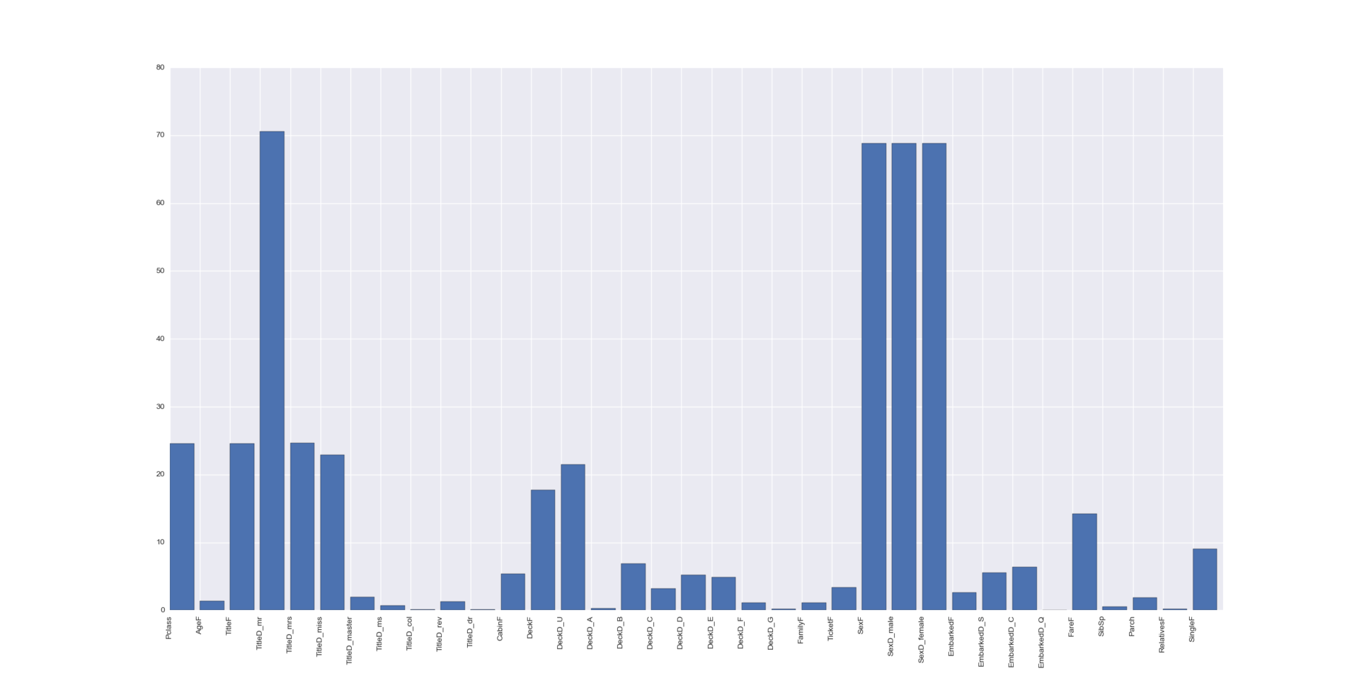
Let us evaluate the importance of our features using the SelectKBest algorithm.
selector = SelectKBest(f_classif, k=5) selector.fit(train_data_munged[predictors], train_data_munged["Survived"]) scores = -np.log10(selector.pvalues_) plt.bar(range(len(predictors)), scores) plt.xticks(range(len(predictors)), predictors, rotation='vertical') plt.show() Here you have an article describing exactly how he does it. Other strategies can be specified in the SelectKBest parameters.
In principle, we already know everything - gender is very important. Titles are important - but they have a strong correlation with sex. The ticket class is important and in some way the F deck.
Grading grade
Before starting any classification, we need to understand how we will evaluate it. In the case of Kaggle contests, everything is very simple: we just read their rules. In the case of the Titanic, the estimate will be the ratio of the correct classifier ratings to the total number of passengers. In other words, this estimate is called accuracy .
But before sending the classification result for the test sample to an assessment in Kaggle, we would be nice to first understand for ourselves at least the approximate quality of our classifier. To understand this, we can only use train-sampling, since only it contains labeled data. But the question remains - how exactly?
Often in examples you can see something like this:
classifier.fit(train_X, train_y) predict_y = classifier.predict(train_X) return metrics.accuracy_score(train_y, predict_y) That is, we train the classifier on the train-set, after which we check it on it. Undoubtedly, to some extent, this gives a certain assessment of the quality of the classifier’s work, but in general this approach is incorrect. The classifier should not describe the data on which he was trained, but some model that generated this data. Otherwise, the classifier perfectly adapts to the train-sample, when checking it shows excellent results, but when checking on some other data set it merges with a bang. What is called overfitting .
The correct approach would be to divide the available train-set into a number of pieces. We can take a few of them, train the classifier on them, and then check his work for the rest. You can produce this process several times just by shuffling the pieces. In sklearn, this process is called cross-validation .
You can already imagine in your head the cycles that will share data, produce training and assessment, but the trick is that all you need to implement this in sklearn is to determine a strategy.
cv = StratifiedKFold(train_data["Survived"], n_folds=3, shuffle=True, random_state=1) Here we define a rather complicated process: the training data will be divided into three pieces, and the records will fall into each piece in a random way (to level the possible dependence on the order), besides the strategy will track the ratio of classes in each piece to be approximately equal. Thus, we will perform three measurements on pieces 1 + 2 vs 3, 1 + 3 vs 2, 2 + 3 vs 1 - after that we will be able to get an average assessment of the accuracy of the classifier (which will characterize the quality of work), as well as the variance of the assessment (which will be characterize the stability of his work).
Classification
Now let's test the work of various classifiers.
KNeighborsClassifier :
alg_ngbh = KNeighborsClassifier(n_neighbors=3) scores = cross_val_score(alg_ngbh, train_data_scaled, train_data_munged["Survived"], cv=cv, n_jobs=-1) print("Accuracy (k-neighbors): {}/{}".format(scores.mean(), scores.std())) SGDClassifier :
alg_sgd = SGDClassifier(random_state=1) scores = cross_val_score(alg_sgd, train_data_scaled, train_data_munged["Survived"], cv=cv, n_jobs=-1) print("Accuracy (sgd): {}/{}".format(scores.mean(), scores.std())) SVC :
alg_svm = SVC(C=1.0) scores = cross_val_score(alg_svm, train_data_scaled, train_data_munged["Survived"], cv=cv, n_jobs=-1) print("Accuracy (svm): {}/{}".format(scores.mean(), scores.std())) GaussianNB :
alg_nbs = GaussianNB() scores = cross_val_score(alg_nbs, train_data_scaled, train_data_munged["Survived"], cv=cv, n_jobs=-1) print("Accuracy (naive bayes): {}/{}".format(scores.mean(), scores.std())) LinearRegression :
def linear_scorer(estimator, x, y): scorer_predictions = estimator.predict(x) scorer_predictions[scorer_predictions > 0.5] = 1 scorer_predictions[scorer_predictions <= 0.5] = 0 return metrics.accuracy_score(y, scorer_predictions) alg_lnr = LinearRegression() scores = cross_val_score(alg_lnr, train_data_scaled, train_data_munged["Survived"], cv=cv, n_jobs=-1, scoring=linear_scorer) print("Accuracy (linear regression): {}/{}".format(scores.mean(), scores.std())) The linear_scorer method is needed because LinearRegression is a regression that returns any real number. Accordingly, we divide the scale by the border of 0.5 and reduce any numbers to two classes - 0 and 1.
LogisticRegression :
alg_log = LogisticRegression(random_state=1) scores = cross_val_score(alg_log, train_data_scaled, train_data_munged["Survived"], cv=cv, n_jobs=-1, scoring=linear_scorer) print("Accuracy (logistic regression): {}/{}".format(scores.mean(), scores.std())) RandomForestClassifier :
alg_frst = RandomForestClassifier(random_state=1, n_estimators=500, min_samples_split=8, min_samples_leaf=2) scores = cross_val_score(alg_frst, train_data_scaled, train_data_munged["Survived"], cv=cv, n_jobs=-1) print("Accuracy (random forest): {}/{}".format(scores.mean(), scores.std())) I did something like this
Accuracy (k-neighbors): 0.698092031425/0.0111105442611
Accuracy (sgd): 0.708193041526/0.0178870678457
Accuracy (svm): 0.693602693603/0.018027360723
Accuracy (naive bayes): 0.791245791246/0.0244349506813
Accuracy (linear regression): 0.805836139169/0.00839878201296
Accuracy (logistic regression): 0.806958473625/0.0156323100754
Accuracy (random forest): 0.827160493827/0.0063488824349
Random Forest won the algorithm and its dispersion is not bad - it seems it is stable.
Even better
Everything seems to be good and you can send the result, but there is only one muddy moment left: each classifier has its own parameters - how can we understand that we have chosen the best option? Without a doubt, you can sit for a long time and sort through the parameters manually - but what if you entrust this work to a computer?
alg_frst_model = RandomForestClassifier(random_state=1) alg_frst_params = [{ "n_estimators": [350, 400, 450], "min_samples_split": [6, 8, 10], "min_samples_leaf": [1, 2, 4] }] alg_frst_grid = GridSearchCV(alg_frst_model, alg_frst_params, cv=cv, refit=True, verbose=1, n_jobs=-1) alg_frst_grid.fit(train_data_scaled, train_data_munged["Survived"]) alg_frst_best = alg_frst_grid.best_estimator_ print("Accuracy (random forest auto): {} with params {}" .format(alg_frst_grid.best_score_, alg_frst_grid.best_params_)) It turns out even better!
Accuracy (random forest auto): 0.836139169473 with params {'min_samples_split': 6, 'n_estimators': 350, 'min_samples_leaf': 2}
Selection can be made even thinner if there is time and desire - either by changing the parameters, or using a different selection strategy, for example, RandomizedSearchCV .
We try xgboost
Everyone praises xgboost - let's try it too.
ald_xgb_model = xgb.XGBClassifier() ald_xgb_params = [ {"n_estimators": [230, 250, 270], "max_depth": [1, 2, 4], "learning_rate": [0.01, 0.02, 0.05]} ] alg_xgb_grid = GridSearchCV(ald_xgb_model, ald_xgb_params, cv=cv, refit=True, verbose=1, n_jobs=1) alg_xgb_grid.fit(train_data_scaled, train_data_munged["Survived"]) alg_xgb_best = alg_xgb_grid.best_estimator_ print("Accuracy (xgboost auto): {} with params {}" .format(alg_xgb_grid.best_score_, alg_xgb_grid.best_params_)) For some reason, the training hung when using all the cores, so I limited myself to one thread (n_jobs = 1), but in single-threaded mode, training and classification in xgboost works very quickly.
The result is also not bad
Accuracy (xgboost auto): 0.835016835017 with params {'n_estimators': 270, 'learning_rate': 0.02, 'max_depth': 2}
Result
The classifier is selected, the parameters are calculated - it remains to generate the result and send it to Kaggle for review.
alg_test = alg_frst_best alg_test.fit(train_data_scaled, train_data_munged["Survived"]) predictions = alg_test.predict(test_data_scaled) submission = pd.DataFrame({ "PassengerId": test_data["PassengerId"], "Survived": predictions }) submission.to_csv("titanic-submission.csv", index=False) In general, it is worth noting a few points in such competitions, which seemed interesting to me:
- — . ;
- - . - Kaggle;
- — — ;
- . — -, , , ;
- — , . — ? , , — - .
,
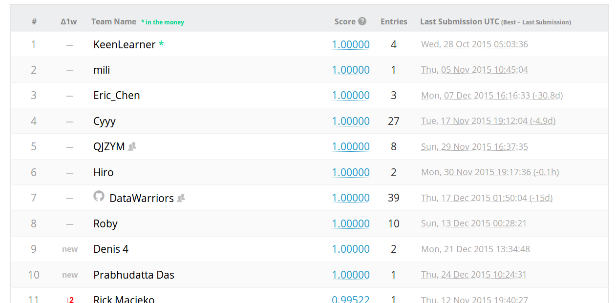
Looking through the top contestants, it is impossible not to notice the people who scored 1 (all the answers are correct) - and some got it from the very first attempt.
The next option comes to mind: someone registered an account with which he began to select (no more than 10 attempts per day are allowed) the correct answers. If I understand correctly, this is a kind of weighing task .
However, after thinking a little more, it is impossible not to smile at our guess: we are talking about a task, the answers for which have long been known! In fact, the death of Titanic was a shock to his contemporaries, and films, books and documentaries were devoted to this event. And most likely somewhere there is a complete list of names of passengers of the Titanic with a description of their fate. But this is no longer true for machine learning.
However, from this it is possible and necessary to draw a conclusion that I am going to apply in the following competitions - not necessarily (if this is not prohibited by the rules of the competition) to be limited only to the data that the organizer issued. For example, by a certain time and place, weather conditions, the state of securities markets, exchange rates, whether the day is a holiday can be identified - in other words, you can marry data from the organizers with any available public data sets that can help in describing the characteristics of the model.
Code
The full script code is here . Do not forget to choose the signs for training.
Source: https://habr.com/ru/post/274171/
All Articles