Recurrent neural network in 10 lines of code appreciated the feedback from viewers of the new episode of “Star Wars”
Hello, Habr! We recently received from Izvestia an order to conduct a public opinion survey on the film Star Wars: The Force Awakens, which premiered on December 17th. To do this, we decided to analyze the tone of the Russian segment of Twitter on several relevant hashtags. The results were expected from us in just 3 days (and this is at the very end of the year!), So we needed a very fast way. We found several similar online services on the Internet (including sentiment140 and tweet_viz ), but it turned out that they do not work with Russian and for some reason analyze only a small percentage of tweets. The AlchemyAPI service would help us, but the limit of 1000 requests per day also did not suit us. Then we decided to make our own blackjack tonality analyzer and the rest, creating a simple recurrent memory neural network. The results of our study were used in the article “Izvestia”, published on January 3.

In this article I will talk a little about this kind of networks and introduce a pair of cool tools for home experiments that will allow even schoolchildren to build neural networks of any complexity with a few lines of code. Welcome under cat.
The main difference between recurrent networks (Recurrent Neural Network, RNN) and traditional networks is the logic of the network, in which each neuron interacts with itself. As a rule, a signal which is some sequence is transmitted to the input of such networks. Each element of such a sequence is alternately transmitted to the same neurons, which return their prediction to themselves along with its next element, until the sequence ends. Such networks, as a rule, are used when working with serial information - mainly with texts and audio / video signals. Elements of the recurrent network are depicted as normal neurons with an additional cyclic arrow, which demonstrates that, in addition to the input signal, the neuron also uses its additional hidden state. If you “expand” such an image, you get a whole chain of identical neurons, each of which receives its own sequence element at the input, produces a prediction and passes it further along the chain as a kind of memory cell. You need to understand that this is an abstraction, because it is one and the same neuron that works out several times in a row.
')

Such a neural network architecture allows solving such tasks as predicting the last word in a sentence, for example the word “sun” in the phrase “the sun shines in a clear sky”.
Modeling memory in a neural network in a similar way introduces a new dimension to the description of its work process — time. Let the neural network receive a sequence of data at the input, for example, a text word by word or a word by letter. Then each next element of this sequence arrives at the neuron at a new conditional point in time. By this time, the neuron already has accumulated experience from the beginning of the arrival of information. In the example of the sun, the vector characterizing the preposition “in” will appear as x 0 , the word “sky” as x 1 and so on. As a result, as h t there should be a vector close to the word "sun".
The main difference between different types of recurrent neurons from each other lies in how the memory cell is processed inside them. The traditional approach involves the addition of two vectors (signal and memory) with the subsequent calculation of the activation of the sum, for example, a hyperbolic tangent. It turns out the usual grid with one hidden layer. A similar scheme is drawn as follows:
But the memory implemented in this way is very short. Since each time the information in memory is mixed with the information in the new signal, after 5-7 iterations, the information is already completely overwritten. Returning to the task of predicting the last word in a sentence, it should be noted that within one sentence such a network will work well, but if it comes to a longer text, the patterns in its beginning will no longer make any contribution to the network’s solutions closer to the end text, as well as the error on the first elements of the sequences in the learning process ceases to contribute to the overall network error. This is a very conditional description of this phenomenon, in fact, it is a fundamental problem of neural networks, which is called the problem of a vanishing gradient , and because of it, the third “winter” of deep learning at the end of the 20th century began when the neural networks were 1.5 decades have lost the lead to support vector machines and boosting algorithms.
To overcome this deficiency, an LSTM-RNN network ( Long Short-Term Memory Recurent Neural Network ) was invented, in which additional internal transformations were added that operate on the memory more carefully. Here is its scheme:
Let's go more in detail on each of the layers:
The first layer calculates how much at this step it needs to forget the previous information — essentially factors to the components of the memory vector.

The second layer calculates how interesting the new information is for it, which came with a signal - the same factor, but for observation.
On the third layer, a linear combination of memory and observation is calculated with only the weights computed for each of the components. This is how a new state of memory is obtained, which is passed on in the same way.
It remains to calculate the output. But since a part of the input signal is already in memory, it is not necessary to consider the activation for the entire signal. First, the signal passes through a sigmoid, which decides which part of it is important for further decisions, then the hyperbolic tangent "smears" the memory vector in the range from -1 to 1, and at the end these two vectors multiply.

The h t and C t thus obtained are transmitted further along the chain. Of course, there are many variations of exactly what activation functions are used by each layer, slightly modify the schemes themselves and so on, but the essence remains the same - first they forget a part of the memory, then they remember a part of the new signal, and then the result is calculated on the basis of this data. I took the pictures from here , there you can also see a few examples of more complex LSTM schemes.
I will not talk here in detail about how such networks are trained, let me just say that the algorithm is used BPTT (Backpropagation Through Time), which is a generalization of the standard algorithm in case there is time on the network. You can read about this algorithm here or here .
Recurrent neural networks built on similar principles are very popular, here are some examples of similar projects:
There are also successful examples of using LSTM grids as one of the layers in hybrid systems. Here is an example of a hybrid network that answers questions on the picture from the “How many books are shown?” Series:

Here the LSTM network works in conjunction with the pattern recognition module in the pictures. Here you can compare different hybrid architectures to solve this problem.
For the Python language, there are many very powerful libraries for creating neural networks. Without aiming to provide at least a complete overview of these libraries, I want to introduce you to the Theano library. Generally speaking, out of the box is a very effective toolkit for working with multidimensional tensors and graphs. Realizations of most algebraic operations on them are available, including the search for extremums of tensor functions, the calculation of derivatives, and so on. And all this can be effectively parallelized and run calculations using CUDA technologies on video cards.
It sounds great if it were not for the fact that Theano itself generates and compiles C ++ code. Maybe this is my prejudice, but I am very suspicious of this kind of systems, because, as a rule, they are filled with an incredible number of bugs that are very difficult to find, perhaps because of this I have not paid enough attention to this library for a long time. But Theano was developed at the Canadian institute MILA under the leadership of Yoshua Bengio, one of the most famous specialists in the field of deep learning of our time, and for my brief experience with it, of course, I did not find any mistakes.
However, Theano is only a library for efficient calculations, you need to independently implement backpropagation, neurons and everything else on it. For example, here is the code using only Theano of the same LSTM network about which I spoke above, and about 650 lines in it, which does not at all correspond to the title of this article. But maybe I would never have tried to work with Theano, if it were not for the amazing library of keras . Being in fact only sugar for the interface of Theano, it just solves the problem stated in the header.
At the core of any code using keras is a model object that describes the order in which and which layers your neural network contains. For example, the model that we used to assess the tonality of Star Wars tweets took as input a sequence of words, so its type was
After declaring the model type, layers are sequentially added to it, for example, you can add an LSTM layer with this command:
After all the layers are added, the model should be compiled, if desired, specifying the type of the loss function, the optimization algorithm and a few more settings:
The compilation takes a couple of minutes, after which the model has clear, fit (), predict (), predict_proba () and evaluate () methods available to everyone. So simple, in my opinion this is an ideal option in order to begin to dive into the depths of deep learning. When the opportunities of keras will be missed and you want, for example, to use your own loss functions, you can go down a level and write a part of the code on Theano. By the way, if programs that other programs generate themselves also frighten someone, you can connect the fresh TensorFlow from Google as a backend to keras, but for now it works much slower.
Let us return to our original task - to determine whether the Russian viewers liked Star Wars or not. I used the simple TwitterSearch library as a handy tool to follow on Twitter search results. Like all open APIs of large systems, Twitter has certain limitations . The library allows you to call a callback after each request, so it is very convenient to arrange pauses. Thus, about 50,000 tweets in Russian were downloaded using the following hashtags:
While they were pumped out, I started searching for a training sample. In English, there are several marked tweet corps in free access, the largest of which is the Stanford training sample of sentiment140 mentioned at the very beginning, and there is also a list of small datasets. But they are all in English, and the task was set specifically for Russian. In this regard, I would like to express a special gratitude to the graduate student (probably already former?) Of the Institute of Informatics Systems named. A.P. Ershova of the SB RAS of Yulia Rubtsova, who laid out the corpus of almost 230,000 marked (with more than 82% accuracy) tweets in open access. There would be more people in our country who donate support the community. In general, they worked with this dataset, you can read about it and download it here .
I cleared all tweets from unnecessary, leaving only continuous sequences of Cyrillic characters and numbers that I drove through PyStemmer . Then I replaced the same words with the same numeric codes, eventually getting a dictionary of about 100,000 words, and tweets presented themselves as sequences of numbers, they are ready for classification. I didn’t clean out the low-frequency garbage, because the grid is smart and would guess that there is too much.
Here is our neural network code on keras:
Except for imports and variable declarations, exactly 10 lines came out, and it could be written in one. Let's run through the code. Online 6 layers:
In order for learning to occur on the GPU when executing this code, you need to set the appropriate flag, for example:
On the GPU, this very model was trained almost 20 times faster than on the CPU - about 500 seconds on dataset of 160,000 tweets (a third of the tweets went for validation).
For such tasks there are no clear rules for the formation of the network topology. We honestly spent half a day experimenting with different configurations, and this one showed the best accuracy - 75%. We compared the result of grid prediction with an ordinary logistic regression, which showed 71% accuracy on the same dataset when text was vectorized using the tf-idf method and about the same 75%, but using tf-idf for bigrams. The reason that the neural network almost did not overtake the logistic regression is most likely because the training sample was still too small (to be honest, such a network requires at least 1 million tweets of the training sample) and is noisy. The training took place in just 1 epoch, since then we fixed a strong retraining.
The model predicted the likelihood of a tweet positive; we considered positive feedback with this probability from 0.65, negative - to 0.45, and the interval between them - neutral. By day, the dynamics are as follows:
In general, it is clear that people liked the film rather. Although I personally do not really :)
I selected 5 examples of tweets from each group (the indicated number is the probability that the feedback is positive):
0.9945:
0.9171:
0.8428:
0.8013:
0.7515:
0.6476:
0.6473:
0.6420:
0.6389:
0.5947:
0.3408:
0.1187:
0.1056:
0.0939:
0.0410:
PS Already after the study was conducted, they came across an article in which they praise convolutional networks for solving this problem. Next time we try them, in keras they are also supported . If one of the readers decides to check himself, write in the comments about the results, it is very interesting. May the Power of Big Data be with you!
In this article I will talk a little about this kind of networks and introduce a pair of cool tools for home experiments that will allow even schoolchildren to build neural networks of any complexity with a few lines of code. Welcome under cat.
What is RNN?
The main difference between recurrent networks (Recurrent Neural Network, RNN) and traditional networks is the logic of the network, in which each neuron interacts with itself. As a rule, a signal which is some sequence is transmitted to the input of such networks. Each element of such a sequence is alternately transmitted to the same neurons, which return their prediction to themselves along with its next element, until the sequence ends. Such networks, as a rule, are used when working with serial information - mainly with texts and audio / video signals. Elements of the recurrent network are depicted as normal neurons with an additional cyclic arrow, which demonstrates that, in addition to the input signal, the neuron also uses its additional hidden state. If you “expand” such an image, you get a whole chain of identical neurons, each of which receives its own sequence element at the input, produces a prediction and passes it further along the chain as a kind of memory cell. You need to understand that this is an abstraction, because it is one and the same neuron that works out several times in a row.
')
Such a neural network architecture allows solving such tasks as predicting the last word in a sentence, for example the word “sun” in the phrase “the sun shines in a clear sky”.
Modeling memory in a neural network in a similar way introduces a new dimension to the description of its work process — time. Let the neural network receive a sequence of data at the input, for example, a text word by word or a word by letter. Then each next element of this sequence arrives at the neuron at a new conditional point in time. By this time, the neuron already has accumulated experience from the beginning of the arrival of information. In the example of the sun, the vector characterizing the preposition “in” will appear as x 0 , the word “sky” as x 1 and so on. As a result, as h t there should be a vector close to the word "sun".
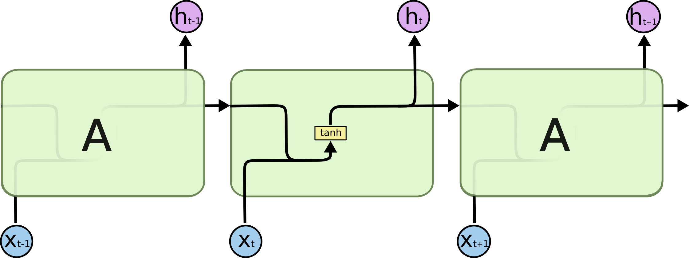
The main difference between different types of recurrent neurons from each other lies in how the memory cell is processed inside them. The traditional approach involves the addition of two vectors (signal and memory) with the subsequent calculation of the activation of the sum, for example, a hyperbolic tangent. It turns out the usual grid with one hidden layer. A similar scheme is drawn as follows:
But the memory implemented in this way is very short. Since each time the information in memory is mixed with the information in the new signal, after 5-7 iterations, the information is already completely overwritten. Returning to the task of predicting the last word in a sentence, it should be noted that within one sentence such a network will work well, but if it comes to a longer text, the patterns in its beginning will no longer make any contribution to the network’s solutions closer to the end text, as well as the error on the first elements of the sequences in the learning process ceases to contribute to the overall network error. This is a very conditional description of this phenomenon, in fact, it is a fundamental problem of neural networks, which is called the problem of a vanishing gradient , and because of it, the third “winter” of deep learning at the end of the 20th century began when the neural networks were 1.5 decades have lost the lead to support vector machines and boosting algorithms.
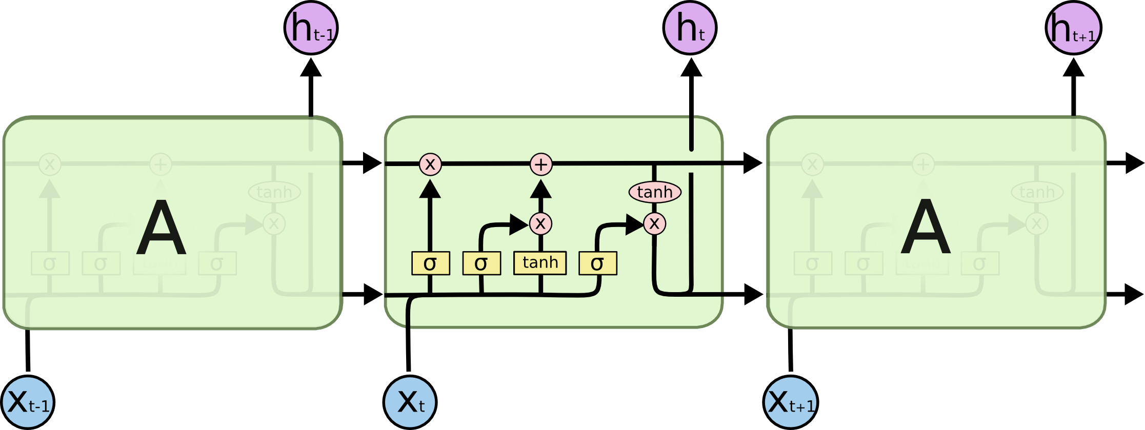
To overcome this deficiency, an LSTM-RNN network ( Long Short-Term Memory Recurent Neural Network ) was invented, in which additional internal transformations were added that operate on the memory more carefully. Here is its scheme:
Let's go more in detail on each of the layers:
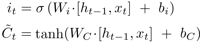
The first layer calculates how much at this step it needs to forget the previous information — essentially factors to the components of the memory vector.
The second layer calculates how interesting the new information is for it, which came with a signal - the same factor, but for observation.
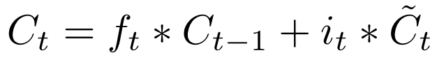
On the third layer, a linear combination of memory and observation is calculated with only the weights computed for each of the components. This is how a new state of memory is obtained, which is passed on in the same way.
It remains to calculate the output. But since a part of the input signal is already in memory, it is not necessary to consider the activation for the entire signal. First, the signal passes through a sigmoid, which decides which part of it is important for further decisions, then the hyperbolic tangent "smears" the memory vector in the range from -1 to 1, and at the end these two vectors multiply.
The h t and C t thus obtained are transmitted further along the chain. Of course, there are many variations of exactly what activation functions are used by each layer, slightly modify the schemes themselves and so on, but the essence remains the same - first they forget a part of the memory, then they remember a part of the new signal, and then the result is calculated on the basis of this data. I took the pictures from here , there you can also see a few examples of more complex LSTM schemes.
I will not talk here in detail about how such networks are trained, let me just say that the algorithm is used BPTT (Backpropagation Through Time), which is a generalization of the standard algorithm in case there is time on the network. You can read about this algorithm here or here .
Using LSTM-RNN
Recurrent neural networks built on similar principles are very popular, here are some examples of similar projects:
There are also successful examples of using LSTM grids as one of the layers in hybrid systems. Here is an example of a hybrid network that answers questions on the picture from the “How many books are shown?” Series:
Here the LSTM network works in conjunction with the pattern recognition module in the pictures. Here you can compare different hybrid architectures to solve this problem.
Theano and keras
For the Python language, there are many very powerful libraries for creating neural networks. Without aiming to provide at least a complete overview of these libraries, I want to introduce you to the Theano library. Generally speaking, out of the box is a very effective toolkit for working with multidimensional tensors and graphs. Realizations of most algebraic operations on them are available, including the search for extremums of tensor functions, the calculation of derivatives, and so on. And all this can be effectively parallelized and run calculations using CUDA technologies on video cards.
It sounds great if it were not for the fact that Theano itself generates and compiles C ++ code. Maybe this is my prejudice, but I am very suspicious of this kind of systems, because, as a rule, they are filled with an incredible number of bugs that are very difficult to find, perhaps because of this I have not paid enough attention to this library for a long time. But Theano was developed at the Canadian institute MILA under the leadership of Yoshua Bengio, one of the most famous specialists in the field of deep learning of our time, and for my brief experience with it, of course, I did not find any mistakes.
However, Theano is only a library for efficient calculations, you need to independently implement backpropagation, neurons and everything else on it. For example, here is the code using only Theano of the same LSTM network about which I spoke above, and about 650 lines in it, which does not at all correspond to the title of this article. But maybe I would never have tried to work with Theano, if it were not for the amazing library of keras . Being in fact only sugar for the interface of Theano, it just solves the problem stated in the header.
At the core of any code using keras is a model object that describes the order in which and which layers your neural network contains. For example, the model that we used to assess the tonality of Star Wars tweets took as input a sequence of words, so its type was
model = Sequential() After declaring the model type, layers are sequentially added to it, for example, you can add an LSTM layer with this command:
model.add(LSTM(64)) After all the layers are added, the model should be compiled, if desired, specifying the type of the loss function, the optimization algorithm and a few more settings:
model.compile(loss='binary_crossentropy', optimizer='adam', class_mode="binary") The compilation takes a couple of minutes, after which the model has clear, fit (), predict (), predict_proba () and evaluate () methods available to everyone. So simple, in my opinion this is an ideal option in order to begin to dive into the depths of deep learning. When the opportunities of keras will be missed and you want, for example, to use your own loss functions, you can go down a level and write a part of the code on Theano. By the way, if programs that other programs generate themselves also frighten someone, you can connect the fresh TensorFlow from Google as a backend to keras, but for now it works much slower.
Tweet analysis
Let us return to our original task - to determine whether the Russian viewers liked Star Wars or not. I used the simple TwitterSearch library as a handy tool to follow on Twitter search results. Like all open APIs of large systems, Twitter has certain limitations . The library allows you to call a callback after each request, so it is very convenient to arrange pauses. Thus, about 50,000 tweets in Russian were downloaded using the following hashtags:
- #starwars
- #star Wars
- #star #wars
- #star Wars
- # AwakeningPower
- #TheForceAwakens
- # awakening # force
While they were pumped out, I started searching for a training sample. In English, there are several marked tweet corps in free access, the largest of which is the Stanford training sample of sentiment140 mentioned at the very beginning, and there is also a list of small datasets. But they are all in English, and the task was set specifically for Russian. In this regard, I would like to express a special gratitude to the graduate student (probably already former?) Of the Institute of Informatics Systems named. A.P. Ershova of the SB RAS of Yulia Rubtsova, who laid out the corpus of almost 230,000 marked (with more than 82% accuracy) tweets in open access. There would be more people in our country who donate support the community. In general, they worked with this dataset, you can read about it and download it here .
I cleared all tweets from unnecessary, leaving only continuous sequences of Cyrillic characters and numbers that I drove through PyStemmer . Then I replaced the same words with the same numeric codes, eventually getting a dictionary of about 100,000 words, and tweets presented themselves as sequences of numbers, they are ready for classification. I didn’t clean out the low-frequency garbage, because the grid is smart and would guess that there is too much.
Here is our neural network code on keras:
from keras.preprocessing import sequence from keras.utils import np_utils from keras.models import Sequential from keras.layers.core import Dense, Dropout, Activation from keras.layers.embeddings import Embedding from keras.layers.recurrent import LSTM max_features = 100000 maxlen = 100 batch_size = 32 model = Sequential() model.add(Embedding(max_features, 128, input_length=maxlen)) model.add(LSTM(64, return_sequences=True)) model.add(LSTM(64)) model.add(Dropout(0.5)) model.add(Dense(1)) model.add(Activation('sigmoid')) model.compile(loss='binary_crossentropy', optimizer='adam', class_mode="binary") model.fit( X_train, y_train, batch_size=batch_size, nb_epoch=1, show_accuracy=True ) result = model.predict_proba(X) Except for imports and variable declarations, exactly 10 lines came out, and it could be written in one. Let's run through the code. Online 6 layers:
- The Embedding layer, which prepares features, the settings indicate that there are 100,000 different features in the dictionary, and the grid should wait for a sequence of no more than 100 words.
- Then, two LSTM layers, each of which outputs a tensor dimension of batch_size / length of a sequence / units in LSTM, and the second gives a matrix of batch_size / units in LSTM. To make the second one understand the first one, the return_sequences = True flag is set.
- The dropout layer is responsible for retraining. It resets the random half of features and prevents co-adaptation of scales in layers (we believe the Canadians to use the word).
- Dense-layer is a normal linear unit, which weightedly summarizes the components of the input vector.
- The last activation layer pushes this value in the interval from 0 to 1 so that it becomes a probability. In essence, Dense and Activation in this order is a logistic regression.
In order for learning to occur on the GPU when executing this code, you need to set the appropriate flag, for example:
THEANO_FLAGS=mode=FAST_RUN,device=gpu,floatX=float32 python myscript.py On the GPU, this very model was trained almost 20 times faster than on the CPU - about 500 seconds on dataset of 160,000 tweets (a third of the tweets went for validation).
For such tasks there are no clear rules for the formation of the network topology. We honestly spent half a day experimenting with different configurations, and this one showed the best accuracy - 75%. We compared the result of grid prediction with an ordinary logistic regression, which showed 71% accuracy on the same dataset when text was vectorized using the tf-idf method and about the same 75%, but using tf-idf for bigrams. The reason that the neural network almost did not overtake the logistic regression is most likely because the training sample was still too small (to be honest, such a network requires at least 1 million tweets of the training sample) and is noisy. The training took place in just 1 epoch, since then we fixed a strong retraining.
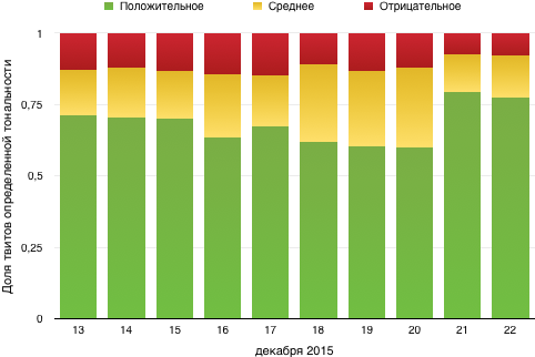
The model predicted the likelihood of a tweet positive; we considered positive feedback with this probability from 0.65, negative - to 0.45, and the interval between them - neutral. By day, the dynamics are as follows:
In general, it is clear that people liked the film rather. Although I personally do not really :)
Network examples
I selected 5 examples of tweets from each group (the indicated number is the probability that the feedback is positive):
Positive tonality
0.9945:
You can breathe out calmly, the new Star Wars are old school excellent. Abrams - cool, as always. Scenario, music, actors and filming - perfect. - snowdenny (@maximlupashko) December 17, 2015
0.9171:
I advise everyone to go to star wars super film— Nikolay (@ shans9494) December 22, 2015
0.8428:
POWER WAKE UP! YES WILL ARRIVE WITH YOU THE POWER OF TODAY AT THE PREMIER OF THE MIRACLE THAT YOU WAITED FOR 10 YEARS! #TheForceAwakens #StarWars - Vladislav Ivanov (@Mrrrrrr_J) December 16, 2015
0.8013:
Although I am not a fan of #StarWars , but this performance is wonderful! #StarWarsForceAwakens https://t.co/1hHKdy0WhB - Oksana Storozhuk (@atn_Oksanasova) December 16, 2015
0.7515:
Who looked star wars today? I am I :)) - Anastasiya Ananich (@NastyaAnanich) December 19, 2015
Mixed pitch
0.6476:
New Star Wars is better than the first episode, but worse than all the others - Igor Larionov (@ Larionovll1013) December 19, 2015
0.6473:
plot spoiler
Han Solo will die. Enjoy watching. #starwars - Nick Silicone (@nicksilicone) December 16, 2015
0.6420:
All around Star Wars. Am I alone in the subject? : / - Olga (@dlfkjskdhn) December 19, 2015
0.6389:
To go or not to go to Star Wars, that is the question - annet_p (@anitamaksova) December 17, 2015
0.5947:
Star Wars left a double impression. And not very good. In some places it was not felt that they were the very ... something alien was slipping— Kolot Eugene (@ KOLOT1991) December 21, 2015
Negative tonality
0.3408:
There are so many conversations around, are I really not a fan of Star Wars? #StarWars #StarWarsTheForceAwakens - modern mind (@ modernmind3) December 17, 2015
0.1187:
they pulled my poor heart out of my chest and shattered it into millions and millions of fragments. #StarWars - Remi Evans (@Remi_Evans) December 22, 2015
0.1056:
I hate the knock-outs, I got star wars from me - the nayla's pajamas (@harryteaxxx) December 17, 2015
0.0939:
I woke up and realized that the new Star Wars was disappointing. - Tim Frost (@Tim_Fowl) December 20, 2015
0.0410:
I am disappointed # waking up the force - Eugenjkee; Star Wars (@eugenjkeee) December 20, 2015
PS Already after the study was conducted, they came across an article in which they praise convolutional networks for solving this problem. Next time we try them, in keras they are also supported . If one of the readers decides to check himself, write in the comments about the results, it is very interesting. May the Power of Big Data be with you!
Source: https://habr.com/ru/post/274027/
All Articles