Static time analysis demystified
Many novice developers of FPGA (and ASIC) do not fully understand the effect of temporal constraints (constraints - hereinafter referred to as constraints) on the synthesis results; the way in which constraints are used in static time analysis. Most of the literature on this topic comes down to the consideration of various types of constraints, but says nothing about the internal “kitchen” and the algorithms used. Consideration of constraints devoted and a recent post on this topic on GT ( geektimes.ru/post/254932/ [1]). Meanwhile, constraints are just the tip of the iceberg. Their use should be based on the fundamental knowledge of static time analysis, which is given, for example, in American universities, but they do not tell us anything. Therefore, actually, let's talk about the foundation.
In modern routes of designing synchronous circuits, two main types of analysis are used: time modeling, and static time analysis.
Temporary modeling is used for the most part for functional verification, and relies on verilog-models of logic elements using plug-in delays (files in sdf, tlf standards, etc.). The advantage of temporal modeling is accuracy, and the ability to model large circuits. Accuracy is certainly lower than when modeling at the level of transistors (spice-modeling), but at the same time it is quite acceptable, and most importantly, orders of magnitude faster. The disadvantage of temporal modeling is the enormous resource consumption of checking the full coverage of circuit logic tests. And most often, 100% coverage of the logic of tests cannot be achieved.
Static time analysis does not simulate the behavior of the circuit in dynamics, and does not use verilog-models of elements. Also, static analysis does not deal with the functions of the circuit and its constituent elements. The main task of the static analysis is to consider all (under 100% of possible combinations) signal delays in the circuit, and to look for violations in accordance with the specified inspection rules (constraints). Static analysis is named because it is produced in statics, according to the connection graph constructed in accordance with the scheme. Or, more precisely, on an acyclic digraph.
')
Without getting into the theory of graphs, it suffices to say that the digraph is a directed graph, i.e. The arcs of the graph have a direction (just as the signal in the wire “runs” in one direction - from the source to the receiver). Arcs of the graph are wires between elements, and “virtual” signal paths (arcs - arches) inside the elements. For example, element 2IL or NOT has only two arches: from each of the inputs to the output. The vertices of the graph are the inputs and outputs of the elements, as well as the inputs and outputs of the circuit. As a result, using the resulting graph, you can build signal paths that run along the arcs of the graph through its vertices. If all possible signal paths are finite, then the graph is called acyclic. Static time analysis works only with acyclic digraphs, and as a result, only with final trajectories of signals. For example, if the circuit contains feedback, part of the signal paths will be looped around and cannot be analyzed. To combat feedbacks, a crutch is used - CAD can try to make the graph acyclic by throwing out one or more arcs from it (as a rule, these are arcs inside the elements). As a result, a graph without feedbacks will be obtained, but the arcs ejected are no longer involved in the analysis — their delay is not taken into account in the calculations.
For a better understanding of what has been said, I will comment on selected slides from lectures on static time analysis, which are read to students of the University of Texas at Austin.
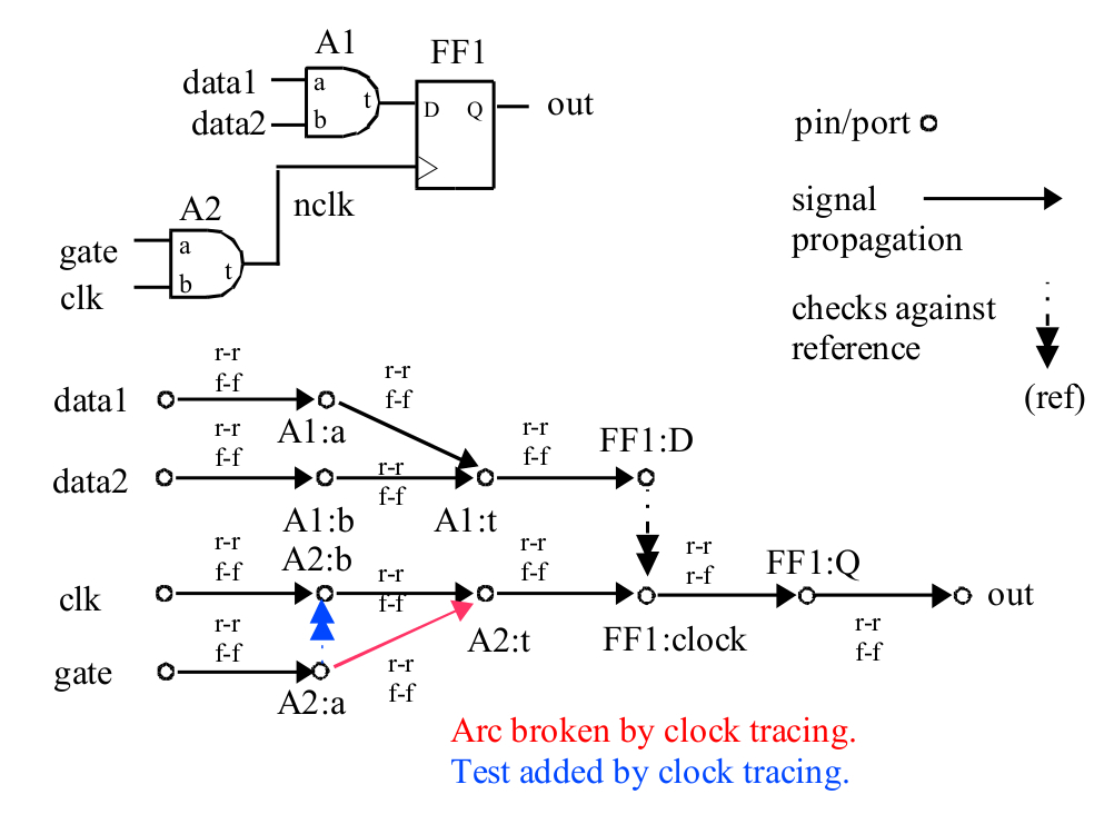
The upper left corner is a scheme consisting of a D-flip-flop (flop), a clock-gate deactivation element, and a logic element at the flop's input. The upper right corner - the rules for constructing a graph:
• circles denote the inputs and outputs of the elements, as well as the inputs and outputs of the circuit,
• arrows show graph edges: wiring and arches (inside elements)
• double arrows with a dotted line indicate the so-called control arches: they do not contain a delay, and in static analysis they are used not for calculating signal delays, but for control - for example, setting and holding signals (setup / hold).
At the bottom of the figure shows the resulting graph. All vertices are signed (it is easy to find a match with the scheme). All arcs are marked as inverting or non-inverting: for example, “rr” and “ff” is decoded as rise-rise and fall-fall, and means that the arc shown does not carry signal inversion. If the arc (for example, the arch in the OR-NOT element) were inverting, then the mark would be “rf” and “fr”, which means rise-fall and fall-rise, or, in other words, a change of the positive signal front during the passage through the arc to the negative, and vice versa. As already mentioned, the function of the elements in the static analysis is not considered, it is only important - the isotonic (non-inverting) function of the element, or the antiton (inverting) function.
What should pay attention. The starting point of the signal path (the essence of the transition process) in synchronous circuits is always either an interface signal or a clock pulse. If the circuit in the above example were larger, then a whole bunch of arcs on the graph would come out of the clock input (clk). And the end point of the signal path in the synchronous scheme is, again, the interface, either - the trigger data input, or the clock-gate resolution. In this case, the end point of the signal path ends with one or more control arches, which indicate which checks for the received signal must be carried out. In the above example, the setup and hold (setup and hold) of the signal at the information input of the trigger is checked against the clock input (FF1: D - FF1: clock), and a similar test of the enable signal of the clock-gate element.
How constraints are reflected on the graph. The constraints affecting the interface delay ( set_input_delay, set_output_delay, set_drive, set_load , etc.) simply change the delay value of the external arcs of the graph. There are constraints that change the graph, for example: set_disable_timing or set_false_path . Many sets are taken automatically from the library of elements: for example, for control arches, check for setup / hold. I don’t want to concentrate on constraints, to understand them, it’s enough to read the description in the documentation of the same Synopsys DC [2], or educational articles on the Internet, for example, on edacafe or semiwiki .
Now about the algorithms for calculating delays. Static time analysis considers only the two extreme points of the spread of delays in the elements and the circuit: the worst case used for checking the constraints on the setup time of a signal (setup) with respect to the clock pulse, and the best case used for checking the hold time. There is still the so-called. Static Statistical Time Analysis (SSTA), which is more intellectually relevant to the question, but about it some other time (especially since this kind of analysis is not relevant at all to FPGA developers).
When calculating delays, two strategies are used - the calculation of the actual arrival time of the signal (AT - Arrival Time), and the calculation based on the required arrival time of the signal (RAT - Required Arrival Time). First, how is AT counted:
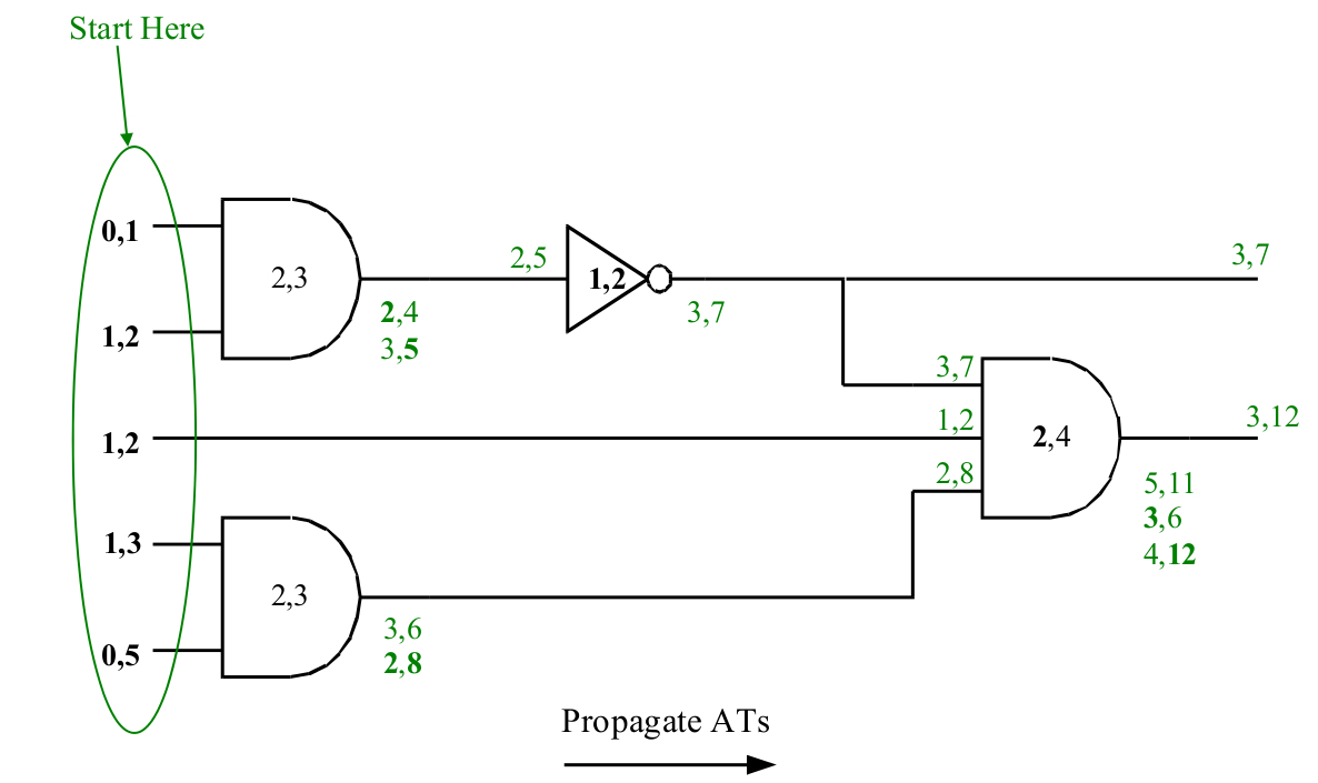
For simplicity, we will assume that the front and rear edge delays are the same (although usually separate calculations are carried out for both options). And instead of the graph, we will draw delays right on the diagram, since this is clearer. Total, in the above figure, the delays of wires are taken into account in the delays of the elements, and are indicated by two digits separated by commas: the first digit indicates the earliest arrival of the signal, and the second digit indicates the latest moment of its arrival. For example, “1.2” at the input means that the signal will come no earlier than 1 ns, and no later than 2 ns, and “2.3” inside the logical element means its delay in the range from 2 to 3 ns. Where in the calculation could take the delay on the input signal? For example, it can be set by set_input_delay with the -min and -max keys. The element delay is taken from the element library (measured by the library developer). Green numbers show the progress of the calculation. For the upper left element - with its own delay of 2-3ns, the output signal can be received at the time of 2-4ns (if the element operates on the first input), and 3-5ns, if on the second. Both ranges simply add up (since the function of the elements is not taken into account), and the result is: “2.5” or from 2 to 5 ns (ie, not earlier than 2 ns, and not later than 5 ns).
Further, on the calculation of the required time:
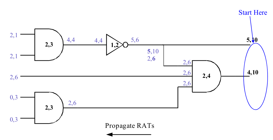
Now the calculation is carried out in the opposite direction. Suppose that the arrival of output signals is limited in the range of “5.10” and “4.10” respectively. These restrictions can be set using set_output_delay with the -min and –max keys. Then there is a calculation in the opposite direction, for example, if from the range of 4-10 subtract the delay of the element 2-4, this will mean that the signal can get to the inputs of the element not earlier than 2 ns and not later than 6 ns. At the same time, the output of the inverter, which had limitations of 5-10, is automatically limited to a more rigid range of 5-6 (obtained by the intersection of 5-10 and 2-6).
In the end, when the required signal propagation time is received, and the actual, it is possible to calculate the violation (slack).
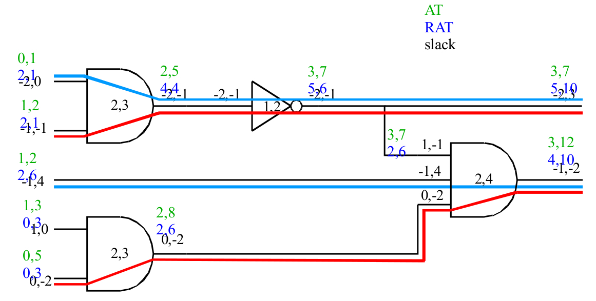
Green shows actual time, blue required. The difference (slack) is calculated, and is shown on the chart in black font. At the same time, a negative difference value is considered a violation, a positive one is considered a margin. In any report of the results of static analysis, you will see two tables - the calculation of the actual time, the calculation of the required, the calculation of the difference, and summing up - MET or NOT MET .
In conclusion, I would like to add that the successful results of the static time analysis are not at all a guarantee of the efficiency of the design. This is indicated by the simple fact that the graph is built with the active participation of the developer (by means of the constraints), and can be constructed with an error. Error in the graph is poured into uncontrolled paths in the scheme, which can be caught only by temporal modeling with checks of time constraints (i.e., using delays at the interfaces). Violation of temporal modeling often indicates an error in the constraints. Hence a simple conclusion - static time analysis does not replace functional modeling, but complements.
I hope the material presented will allow you to better understand the static time analysis, to see it “from the inside,” and more intelligently write the constraints for your design. For those who want to dig further, I can advise you to read the book “Static Timing Analysis for Nanometer: A Practical Approach” [3] in English.
[1] geektimes.ru/post/254932/
[2] www.synopsys.com
[3] www.springer.com/us/book/9780387938196
In modern routes of designing synchronous circuits, two main types of analysis are used: time modeling, and static time analysis.
Temporary modeling is used for the most part for functional verification, and relies on verilog-models of logic elements using plug-in delays (files in sdf, tlf standards, etc.). The advantage of temporal modeling is accuracy, and the ability to model large circuits. Accuracy is certainly lower than when modeling at the level of transistors (spice-modeling), but at the same time it is quite acceptable, and most importantly, orders of magnitude faster. The disadvantage of temporal modeling is the enormous resource consumption of checking the full coverage of circuit logic tests. And most often, 100% coverage of the logic of tests cannot be achieved.
Static time analysis does not simulate the behavior of the circuit in dynamics, and does not use verilog-models of elements. Also, static analysis does not deal with the functions of the circuit and its constituent elements. The main task of the static analysis is to consider all (under 100% of possible combinations) signal delays in the circuit, and to look for violations in accordance with the specified inspection rules (constraints). Static analysis is named because it is produced in statics, according to the connection graph constructed in accordance with the scheme. Or, more precisely, on an acyclic digraph.
')
Without getting into the theory of graphs, it suffices to say that the digraph is a directed graph, i.e. The arcs of the graph have a direction (just as the signal in the wire “runs” in one direction - from the source to the receiver). Arcs of the graph are wires between elements, and “virtual” signal paths (arcs - arches) inside the elements. For example, element 2IL or NOT has only two arches: from each of the inputs to the output. The vertices of the graph are the inputs and outputs of the elements, as well as the inputs and outputs of the circuit. As a result, using the resulting graph, you can build signal paths that run along the arcs of the graph through its vertices. If all possible signal paths are finite, then the graph is called acyclic. Static time analysis works only with acyclic digraphs, and as a result, only with final trajectories of signals. For example, if the circuit contains feedback, part of the signal paths will be looped around and cannot be analyzed. To combat feedbacks, a crutch is used - CAD can try to make the graph acyclic by throwing out one or more arcs from it (as a rule, these are arcs inside the elements). As a result, a graph without feedbacks will be obtained, but the arcs ejected are no longer involved in the analysis — their delay is not taken into account in the calculations.
For a better understanding of what has been said, I will comment on selected slides from lectures on static time analysis, which are read to students of the University of Texas at Austin.
The upper left corner is a scheme consisting of a D-flip-flop (flop), a clock-gate deactivation element, and a logic element at the flop's input. The upper right corner - the rules for constructing a graph:
• circles denote the inputs and outputs of the elements, as well as the inputs and outputs of the circuit,
• arrows show graph edges: wiring and arches (inside elements)
• double arrows with a dotted line indicate the so-called control arches: they do not contain a delay, and in static analysis they are used not for calculating signal delays, but for control - for example, setting and holding signals (setup / hold).
At the bottom of the figure shows the resulting graph. All vertices are signed (it is easy to find a match with the scheme). All arcs are marked as inverting or non-inverting: for example, “rr” and “ff” is decoded as rise-rise and fall-fall, and means that the arc shown does not carry signal inversion. If the arc (for example, the arch in the OR-NOT element) were inverting, then the mark would be “rf” and “fr”, which means rise-fall and fall-rise, or, in other words, a change of the positive signal front during the passage through the arc to the negative, and vice versa. As already mentioned, the function of the elements in the static analysis is not considered, it is only important - the isotonic (non-inverting) function of the element, or the antiton (inverting) function.
What should pay attention. The starting point of the signal path (the essence of the transition process) in synchronous circuits is always either an interface signal or a clock pulse. If the circuit in the above example were larger, then a whole bunch of arcs on the graph would come out of the clock input (clk). And the end point of the signal path in the synchronous scheme is, again, the interface, either - the trigger data input, or the clock-gate resolution. In this case, the end point of the signal path ends with one or more control arches, which indicate which checks for the received signal must be carried out. In the above example, the setup and hold (setup and hold) of the signal at the information input of the trigger is checked against the clock input (FF1: D - FF1: clock), and a similar test of the enable signal of the clock-gate element.
How constraints are reflected on the graph. The constraints affecting the interface delay ( set_input_delay, set_output_delay, set_drive, set_load , etc.) simply change the delay value of the external arcs of the graph. There are constraints that change the graph, for example: set_disable_timing or set_false_path . Many sets are taken automatically from the library of elements: for example, for control arches, check for setup / hold. I don’t want to concentrate on constraints, to understand them, it’s enough to read the description in the documentation of the same Synopsys DC [2], or educational articles on the Internet, for example, on edacafe or semiwiki .
Now about the algorithms for calculating delays. Static time analysis considers only the two extreme points of the spread of delays in the elements and the circuit: the worst case used for checking the constraints on the setup time of a signal (setup) with respect to the clock pulse, and the best case used for checking the hold time. There is still the so-called. Static Statistical Time Analysis (SSTA), which is more intellectually relevant to the question, but about it some other time (especially since this kind of analysis is not relevant at all to FPGA developers).
When calculating delays, two strategies are used - the calculation of the actual arrival time of the signal (AT - Arrival Time), and the calculation based on the required arrival time of the signal (RAT - Required Arrival Time). First, how is AT counted:
For simplicity, we will assume that the front and rear edge delays are the same (although usually separate calculations are carried out for both options). And instead of the graph, we will draw delays right on the diagram, since this is clearer. Total, in the above figure, the delays of wires are taken into account in the delays of the elements, and are indicated by two digits separated by commas: the first digit indicates the earliest arrival of the signal, and the second digit indicates the latest moment of its arrival. For example, “1.2” at the input means that the signal will come no earlier than 1 ns, and no later than 2 ns, and “2.3” inside the logical element means its delay in the range from 2 to 3 ns. Where in the calculation could take the delay on the input signal? For example, it can be set by set_input_delay with the -min and -max keys. The element delay is taken from the element library (measured by the library developer). Green numbers show the progress of the calculation. For the upper left element - with its own delay of 2-3ns, the output signal can be received at the time of 2-4ns (if the element operates on the first input), and 3-5ns, if on the second. Both ranges simply add up (since the function of the elements is not taken into account), and the result is: “2.5” or from 2 to 5 ns (ie, not earlier than 2 ns, and not later than 5 ns).
Further, on the calculation of the required time:
Now the calculation is carried out in the opposite direction. Suppose that the arrival of output signals is limited in the range of “5.10” and “4.10” respectively. These restrictions can be set using set_output_delay with the -min and –max keys. Then there is a calculation in the opposite direction, for example, if from the range of 4-10 subtract the delay of the element 2-4, this will mean that the signal can get to the inputs of the element not earlier than 2 ns and not later than 6 ns. At the same time, the output of the inverter, which had limitations of 5-10, is automatically limited to a more rigid range of 5-6 (obtained by the intersection of 5-10 and 2-6).
In the end, when the required signal propagation time is received, and the actual, it is possible to calculate the violation (slack).
Green shows actual time, blue required. The difference (slack) is calculated, and is shown on the chart in black font. At the same time, a negative difference value is considered a violation, a positive one is considered a margin. In any report of the results of static analysis, you will see two tables - the calculation of the actual time, the calculation of the required, the calculation of the difference, and summing up - MET or NOT MET .
In conclusion, I would like to add that the successful results of the static time analysis are not at all a guarantee of the efficiency of the design. This is indicated by the simple fact that the graph is built with the active participation of the developer (by means of the constraints), and can be constructed with an error. Error in the graph is poured into uncontrolled paths in the scheme, which can be caught only by temporal modeling with checks of time constraints (i.e., using delays at the interfaces). Violation of temporal modeling often indicates an error in the constraints. Hence a simple conclusion - static time analysis does not replace functional modeling, but complements.
I hope the material presented will allow you to better understand the static time analysis, to see it “from the inside,” and more intelligently write the constraints for your design. For those who want to dig further, I can advise you to read the book “Static Timing Analysis for Nanometer: A Practical Approach” [3] in English.
[1] geektimes.ru/post/254932/
[2] www.synopsys.com
[3] www.springer.com/us/book/9780387938196
Source: https://habr.com/ru/post/273849/
All Articles