Vacation Where? When? R

While outside the window is the temperature on the way to the next record, it is interesting to see which temperatures have occurred at any time interval, for any years over the past few decades, at 30,000 points around the world. But it may not be miscalculated with the days of vacation, and take them on those days when there is some kind of "statistical advantage" in the chosen location due to warm weather, or maybe cold, by evaluating it visually on any of the three types of diagrams. Well, or you can just rotate the globe, visually assess the variety of temperatures and "how beautiful this world is."

Data collection

Data sources were data from weather stations located around the world, the results of which are also provided to the National Oceanic and Atmospheric Administration (NOAA ), on the site of which there is an archive of readings of these stations from 1901 on all ( more than 30 000) stations existing during this time, currently there are about 14 000 actual stations. Access to data is provided via ftp , there are quite a lot of different data (there are average daily and more frequent data, data in each file and They are measured by temperature, humidity, precipitation, wind, etc.); I will use only the data on average daily temperature.
The data for each year for each station is an archived text file with delimiters. The total number of files on this resource, about 700,000, it was possible to download them all, the approximate download time would be about two days and would require about 200 GB of disk space, but I do not see the need for this, since the download time for one unit of data ( one station in one year) is less than 0.2 seconds, so for the vast majority of requests (5-10 stations, in 5-10 years) the waiting time is no more than a minute, therefore online access. Each station has a synoptic index (unique code), name, and coordinates. Unfortunately, the names of the stations are not always informative, but in most cases it is the nearest settlement, in other cases - the airport located nearby. Many stations were closed or vice versa opened recently, so for some years there may be gaps. After selecting the time interval of interest, sampling is performed on this range, charting and displaying averaged data on the globe and on the map.

Display on the globe and on the map

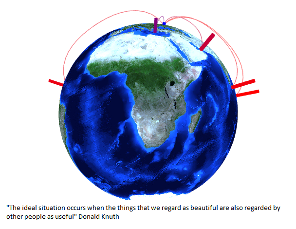
The threejs package is used to display data on a rotating globe. For rendering it is possible to use a graphic format - jpeg file (in geographic projection on the WGS84 ellipsoid) or by generating the object. In this case, a ready jpeg file is used - the land cover of the Blue Marble Next Generation dataset from NASA's site dated August 2004 (8 km resolution per pixel). As a result, since one parameter can be displayed on the globe, the average (median) temperature is displayed on it (both by year and by interval of days). On the globe, for a specific point, a bar of a certain color, height and thickness is displayed, in my case all these parameters are used to display the averaged temperature over all years over the entire time interval of interest relative to all selected stations, scaling is used in the case of bar sizes and transition in color from blue to red for temperatures (that is, for stations with averaged temperatures (-10 °, -5 °, + 7 °, + 10 °, + 30 °) the blue bar with the minimum height and thickness will be for the weather station from -10 °, the red bar with Maximum Feed-height thickness for a weather station to be + 30 °, and the size and color of the remaining stations in proportion calculated with respect to these extreme values).
In addition to these bars, curves from one point (Moscow) are also indicated, they show the trajectories to the selected stations, the thickness and color of these curves are also scaled relative to temperature. The display of these curves clearly shows both the distance and the average temperature. Also, in addition to the data on the globe (which can be rotated and increased), this information (average temperature, distance, and colors used) are given in the adjacent table (Fig. 1). Also, in addition to the globe, the same averaged data is shown on a flat Google map ( Map tab).
')

Charts, static and interactive

The graphical web interface is traditionally the annoying user-friendly shiny-dashboard interface, in which, as seen in the screenshots, parameters are selected in the sidebar, and the main one uses the tabbed panel.

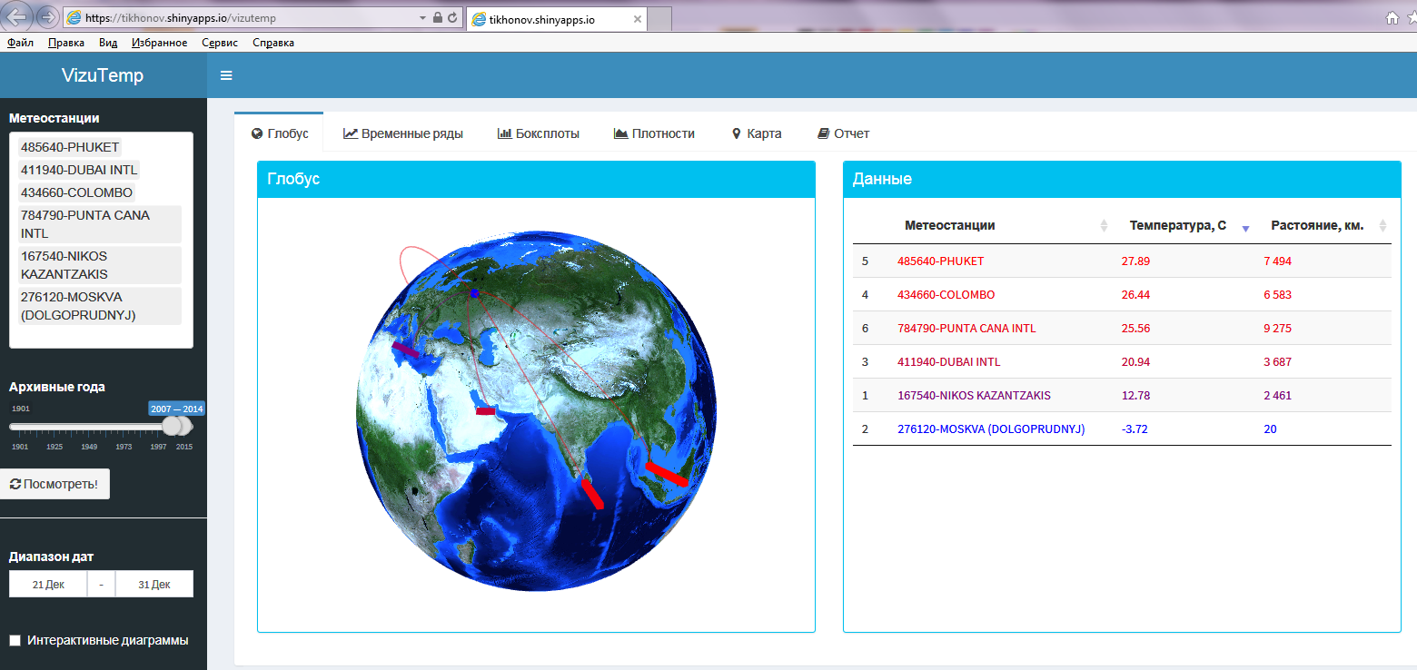
Fig. 1. Main window

In addition to the data on the first tab (on the globe) (which are averaged and do not carry additional information), it is more interesting to look at the variation and temperature dynamics both over the years and relative to each other, the following charts are used for this (tabs), all panel diagrams :
- Time series (Fig. 2) - regular time series, where on each panel (meteorological station) archive years are colored, and the black bold curve is averaged over these years (the figure shows an interactive diagram, the hovering shows a legend by historical temperatures (sorted ) for each day)

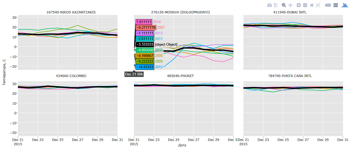
Fig.2. Time series chart

- Boxsplot, scale diagram (Fig. 3) - in this case, every day is considered as atomic and this diagram shows the spread of values ​​on a specific date for all selected years

Fig.3. Span diagram (boxsplat, box with mustache)

- Densities (Fig. 4) - a diagram of temperature densities for selected stations, where the years are already shown on the panels, it clearly shows both the ratios of temperatures by stations and the dynamics of time (by years)

Fig.4. Density chart

In addition to the static ggplot2 charts, by checking the checkbox “interactive charts” the charts are converted to interactive charts that show the legend by hovering, the charts themselves can be enlarged, reduced, moved axes. To do this, transfer existing ggplot2 objects into a direct interactive mapping, using the plotly package.

Preservation

To save all the results, it is possible to unload all the charts and tables in the html format and / or docx ( Report tab). To do this, select the desired format and save the file. Here integration with markdown is used , for this purpose Rmarkdown file layout is used , which contains both plain text and R function call.

Conclusion

As a result, because of my desire to get a “statistical advantage” in choosing the optimal vacation days, it turned out a tool where you can look at the historical temperatures of any interval of days almost anywhere in the world, and evaluate whether there is some globally local warming . Traditionally, thanks to R, all this was implemented fairly quickly and simply.