Apply machine learning to improve PostgreSQL performance.

Machine learning is engaged in the search for hidden patterns in the data. The growing growth of interest in this topic in the IT community is associated with exceptional results obtained through it. Speech recognition and scanned documents, search engines - all this is created using machine learning. In this article I will talk about the current project of our company: how to apply the methods of machine learning to increase the performance of the DBMS.
The first part of this article deals with the existing PostgreSQL scheduler mechanism, the second part describes the possibilities for improving it using machine learning.

')

What is a SQL query execution plan?

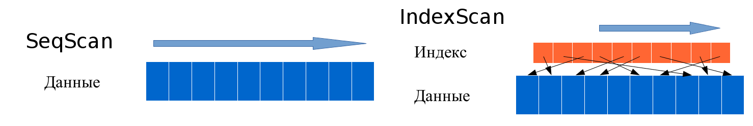
Recall that SQL is a declarative language. This means that the user indicates only what operations should be done with the data. The DBMS is responsible for selecting the method for performing these operations. For example, the query

SELECT name FROM users WHERE age > 25;

You can do it in two ways: read all the records from the users table and check each of them for age> 25, or use the index on the age field. In the second case, we do not view the extra records, but spend more time processing one record due to operations with indices.

Consider a more complex query.

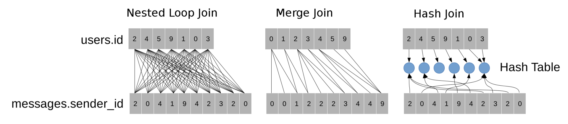
 SELECT messages.text FROM users, messages WHERE users.id = messages.sender_id;

This JOIN can be done in three ways:

A nested loop (NestedLoopJoin) scans all possible pairs of records from two tables and checks the condition for each pair.
Merging (MergeJoin) sorts both tables by the id and sender_id fields, respectively, and then uses the two-pointer method to find all pairs of records that satisfy the condition. This method is similar to the merge sort method (MergeSort).
Hashing (HashJoin) builds a hash table over the field of the smallest table (in our case, this field is users.id). The hash table allows for each record from messages to quickly find a record in which users.id = messages.sender_id.

If the request requires more than one Join operation, then you can also perform them in a different order, for example, in the request

 SELECT u1.name, u2.name, m.text FROM users as u1, messages as m, users as u2 WHERE u1.id = m.sender_id AND u2.id = m.reciever_id;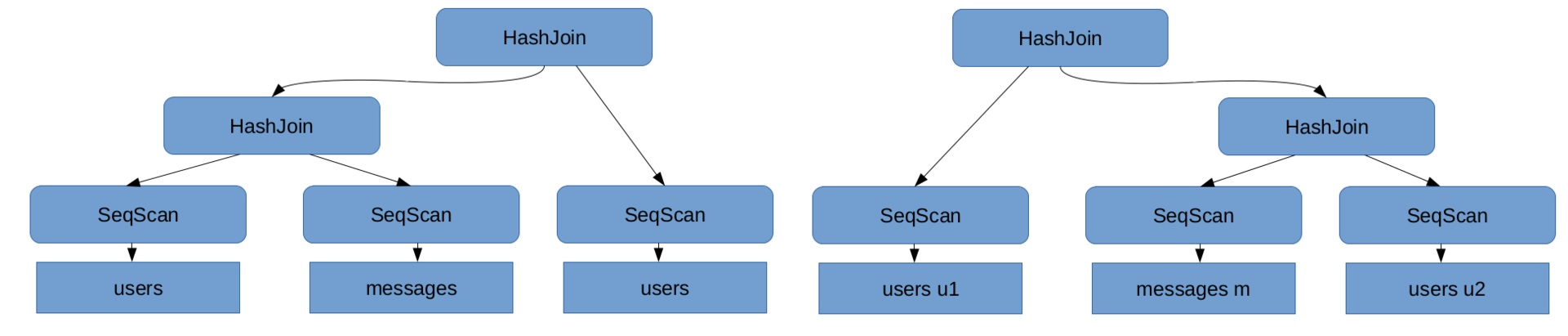

The query execution tree is called the query execution plan .

You can view the plan that the DBMS chooses for a particular request using the explain command:

 EXPLAIN SELECT u1.name, u2.name, m.text FROM users as u1, messages as m, users as u2 WHERE u1.id = m.sender_id AND u2.id = m.reciever_id;

In order to fulfill the request and see the plan chosen for it, you can use the explain analyse command:

 EXPLAIN ANALYSE SELECT u1.name, u2.name, m.text FROM users as u1, messages as m, users as u2 WHERE u1.id = m.sender_id AND u2.id = m.reciever_id;

The execution time of different plans for the same query may differ by many orders of magnitude. Therefore, the correct choice of the query execution plan has a serious impact on the performance of the DBMS. We will understand in more detail how the plan is selected in PostgreSQL now.

How does the DBMS search for the optimal query execution plan?

You can divide the process of finding the optimal plan into two parts.

First, you need to be able to estimate the cost of any plan - the amount of resources necessary for its implementation. In the case when the server does not perform other tasks and requests, the estimated time to complete the request is directly proportional to the amount of resources spent on it. Therefore, we can assume that the cost of the plan is its execution time in some conventional units.

Secondly, you want to choose a plan with a minimum estimate of value. It is easy to show that the number of plans grows exponentially with an increase in the complexity of the query, so you cannot just go through all the plans, estimate the cost of each and choose the cheapest one. To search for the optimal plan, more complex discrete optimization algorithms are used: dynamic programming over subsets for simple queries and a genetic algorithm for complex ones.

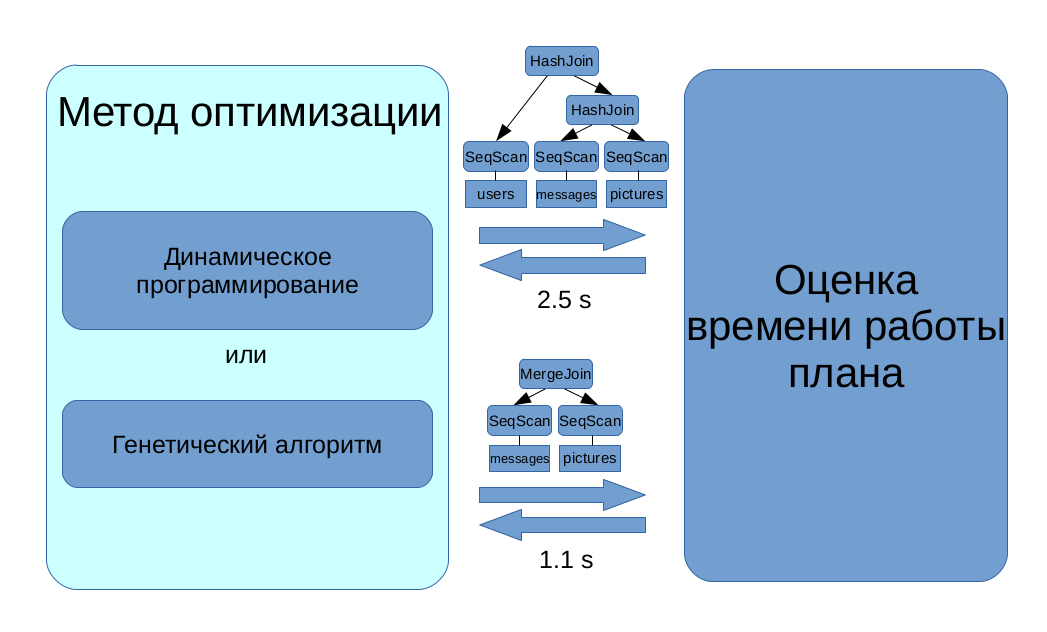
In our project, we focused on the first task: according to this plan, we need to predict its cost. How can this be done without launching a plan for execution?

In fact

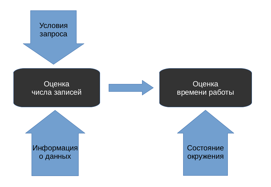
In PostgreSQL, two costs are predicted for the plan: start-up cost and total cost. The start-up cost shows how much resources the plan spends before it issues the first record, and the total cost — how many total resources the plan will need to complete. However, this is not essential for this article. In the future, the cost of implementation will be understood as the total cost.

This task is also divided into two subtasks. First, for each vertex of the plan (plan node) it is predicted how many tuples will be selected in it. Then, on the basis of this information, the cost of executing each vertex, and, accordingly, the entire plan, is estimated.

We did a little research to establish which of the two subtasks in PostgreSQL is worse.
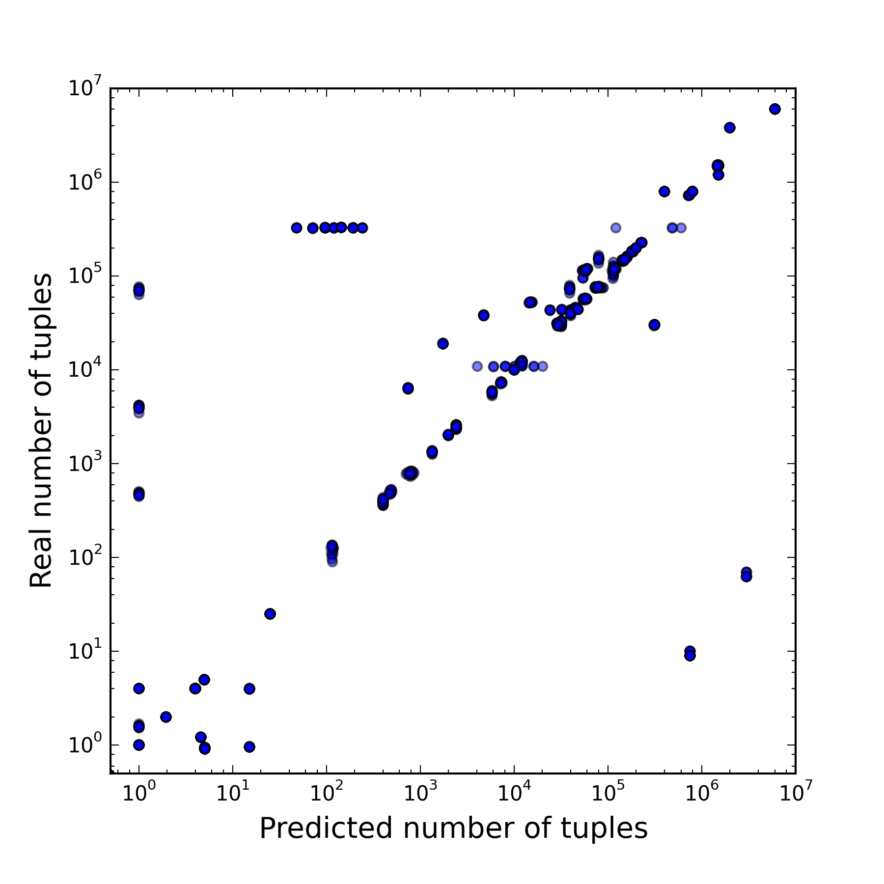
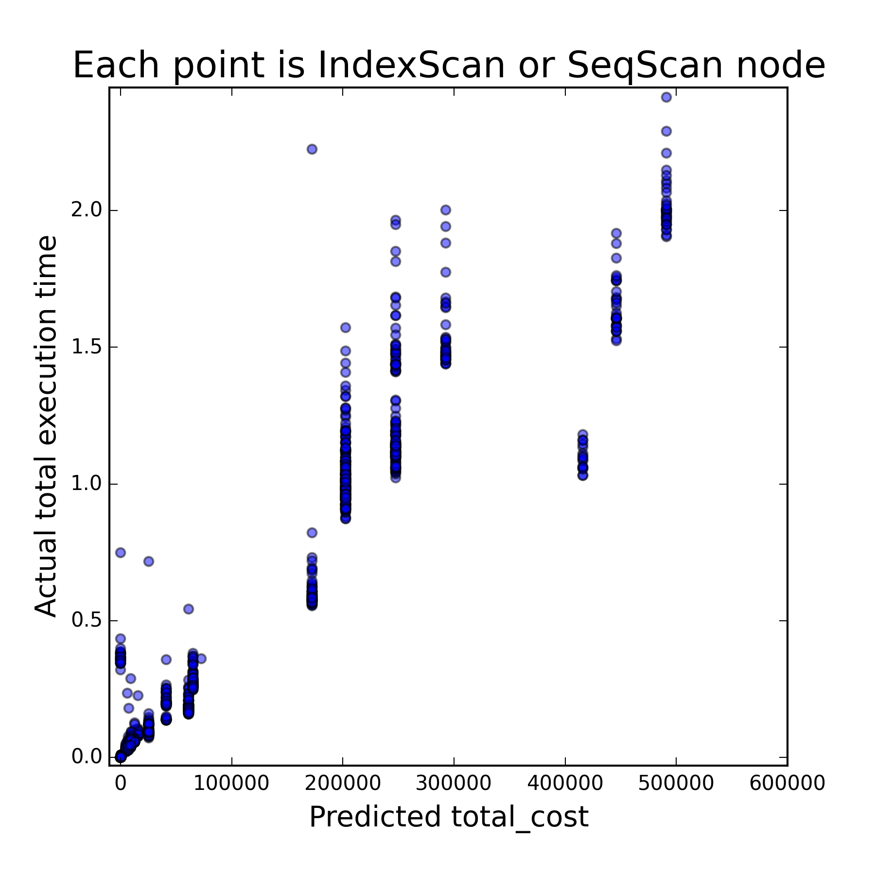
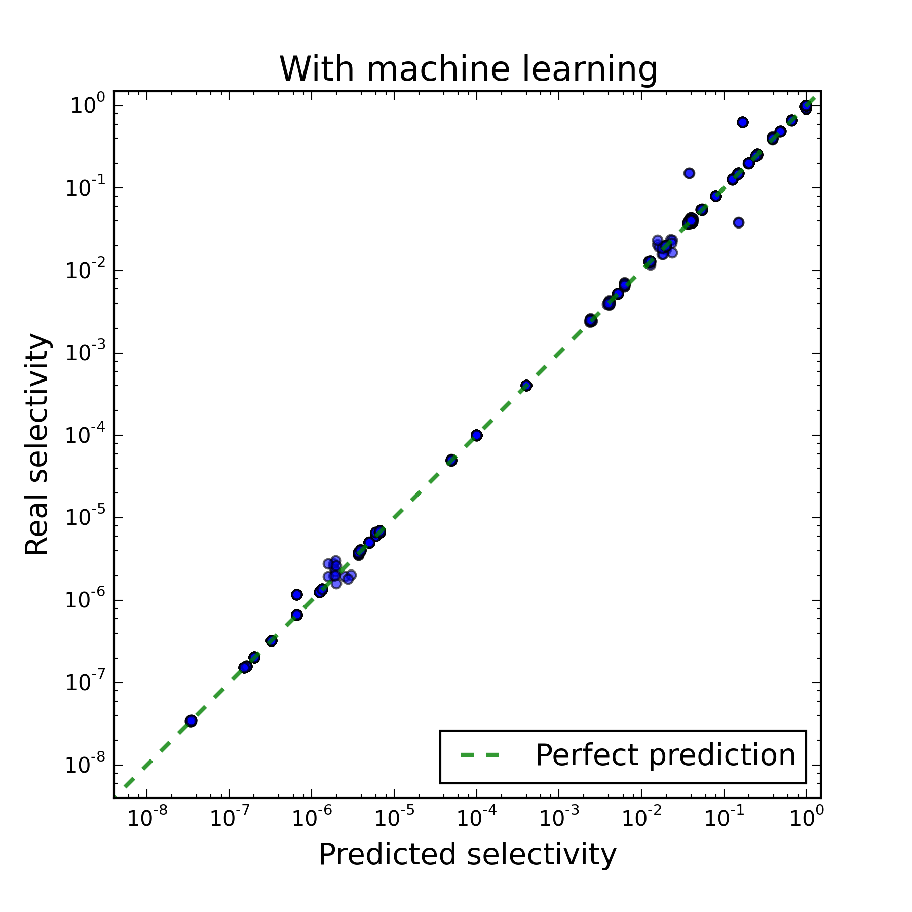
Each point in the figures below corresponds to one vertex of the plan. For each vertex, the number of tuples selected in it and the cost of its execution were predicted, and then the actual number of selected tuples and the execution time were measured. On the right picture, only those vertices are displayed for which the number of tuples is predicted correctly, so it is possible to judge the quality of the cost estimate from it.


Dependence of the true number of tuples on the predicted	The dependence of the time of the plan on the cost if the number of tuples is predicted correctly

The first figure shows that the result of solving the first subtask differs from the true one by several orders of magnitude. The second figure shows that with the right solution to the first subtask, the PostgreSQL model rather adequately estimates the cost of executing one plan or another, since a strong correlation with the execution time is seen. As a result, it was found that the performance of the DBMS suffers from inaccurate solutions of both subtasks, but it suffers more from the incorrectly established number of tuples at each vertex.

Consider the first subtask solution used in PostgreSQL.

How does the DBMS estimate the number of tuples at the vertices?

First, let's try to predict the number of tuples selected by a simple query.

 SELECT name FROM users WHERE age < 25;

In order to have at least some opportunity to do this, we need some information about the data, statistics on them. PostgreSQL uses histograms for this data information.

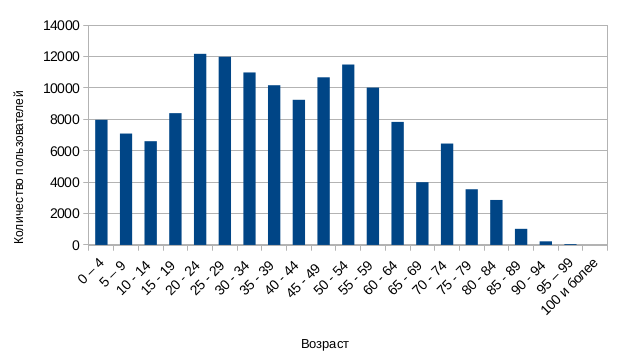
Using the histogram, we can easily restore the proportion of those users who are under 25 years old. For each vertex of the plan, the proportion of all selected tuples in relation to all processed tuples is called selectivity . In the given example, the selectivity of SeqScan will be approximately 0.3. To get the number of tuples selected by the vertex, it will be enough to multiply the vertex selectivity by the number of processed tuples (in the case of SeqScan, this will be the number of records in the table).

Consider a more complex query.

 SELECT name FROM users WHERE age < 25 AND city = 'Moscow';

In this case, using histograms by age and city, we can only get marginal selectivity, that is, the proportion of users under 25 and the proportion of Muscovites among users. In the PostgreSQL model, all conditions (except pairs of conditions like 5 < a AND a < 7 , which automatically turn into condition 5 < a < 7 ) are considered independent . Mathematicians call two conditions A and B independent if the probability that both conditions are fulfilled simultaneously is equal to the product of their probabilities: P (A and B) = P (A) P (B). However, in the applied sense, one can understand the independence of two quantities as the fact that the distribution of another quantity does not depend on the value of one quantity.

What is the problem?

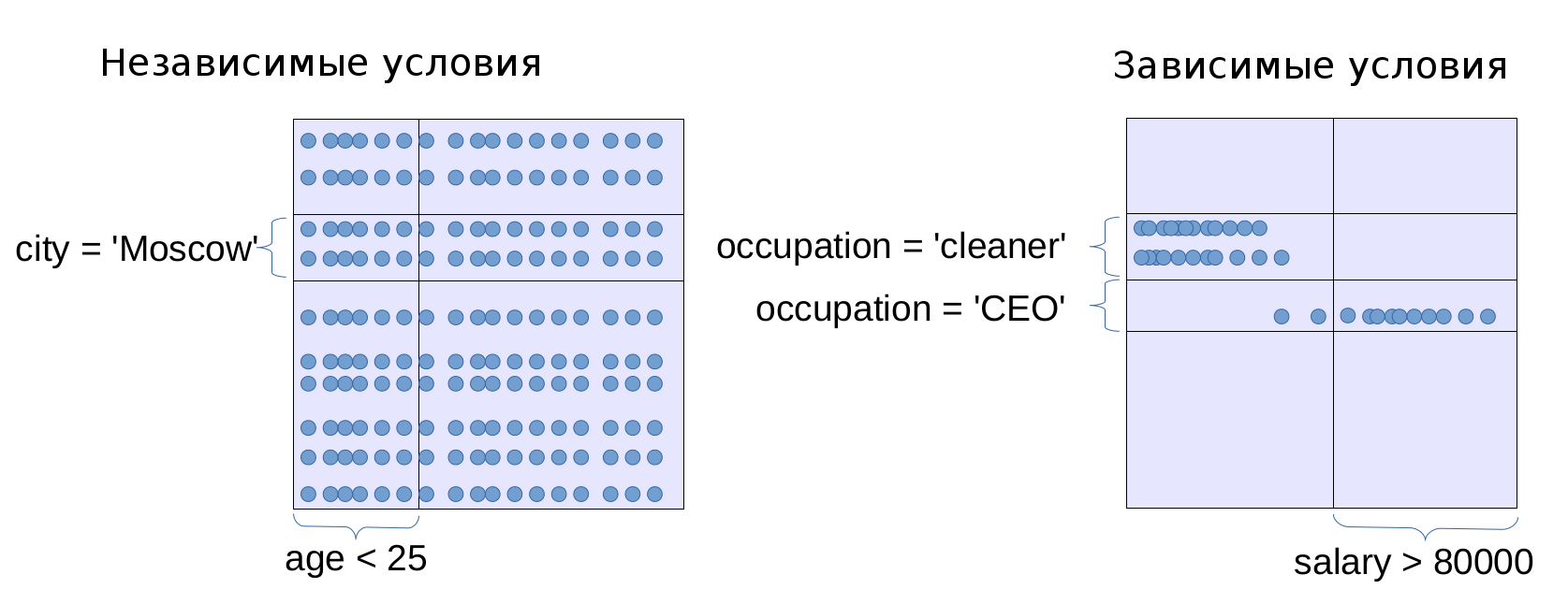
In some cases, the assumption of independence conditions is not satisfied. In such cases, the PostgreSQL model does not work very well. There are two ways to deal with this problem.

The first way is to build multi-dimensional histograms. The problem with this method is that as the dimension increases, a multidimensional histogram requires an exponentially growing amount of resources to maintain the same accuracy. Therefore it is necessary to be limited to histograms of small dimension (2-8 measurements). From here follows the second problem of this method: it is necessary to somehow understand for which pairs (or triples, or quadruples ...) of columns it makes sense to build multidimensional histograms, and for which it is not necessary.
To solve this problem, you need either a good administrator who will study the plans of resource-intensive queries, determine correlations between the columns and manually specify which histograms you need to complete, or a software tool that will try to find columns dependent on each other using statistical tests. However, it does not make sense to build histograms for all dependent columns, therefore the software should also analyze the coexistence of columns in queries. Currently, there are patches that allow using multidimensional histograms in PostgreSQL, but the administrator needs to manually specify in which columns these multidimensional histograms should be built.

We use machine learning to evaluate selectivity.

However, this article focuses on an alternative approach. An alternative approach is the use of machine learning to find the joint selectivity of several conditions. As mentioned above, machine learning is engaged in finding patterns in the data. Data is a collection of objects. In our case, the object is a set of conditions in one vertex of the plan. According to these conditions and their marginal choices, we need to predict joint selectivity.

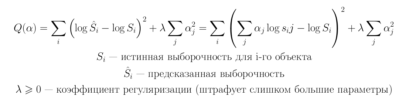
The observed signs of the top of the plan will be the marginal selectivity of all its conditions. We assume that all conditions that differ only in constants are equivalent to each other. You can consider this assumption as a typical method of machine learning - hashing trick - used to reduce the dimension of space. However, a more powerful motivation is behind this: we assume that all the information necessary for a prediction about the constants of a condition is contained in its marginal selectivity. This can be shown strictly for simple conditions of the form a <const: here, by the conditional selectivity, we can restore the value of a constant, that is, there is no loss of information.

The resulting machine learning task will look like the one shown in the figure.

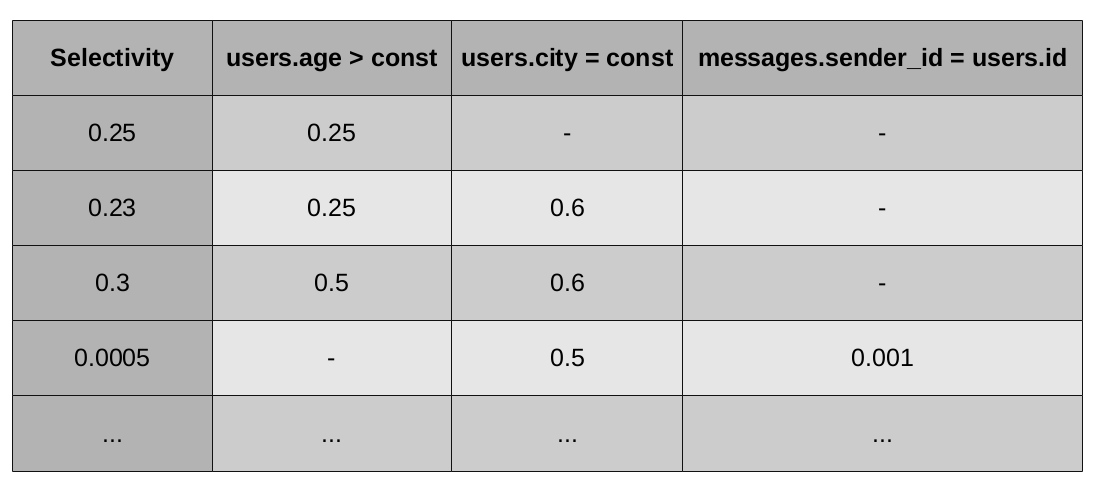
We must predict the leftmost column from the known values in all other columns. Such a task, in which it is necessary to predict a real number, in machine learning is called a regression problem. The method that solves it is called the regressor, respectively.

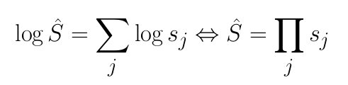
Let us turn to logarithms in all columns. Note that if we now use linear regression, then we will get the current PostgreSQL model as a special case.

Linear regression:

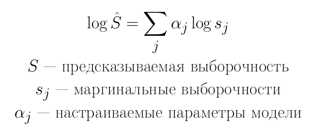
In the case when all the adjustable parameters are 1, we get the standard PostgreSQL selectivity model:

The standard ridge regression method suggests looking for parameters by minimizing the following functional:

To test different approaches, we used the TPC-H benchmark.

The following methods were used as simple regressors:

Ridge linear regression + stochastic gradient descent. This method is good because it allows the use of dynamic learning (online learning), so it does not require to store any observable objects.
Many linear ridge regression + stochastic gradient descent. Here it is assumed that for each set of conditions a separate row-wise linear regressor is created. This method, like the previous one, is good because it allows the use of dynamic learning, so it does not require to store any observable objects, but it works somewhat more precisely than the previous one, because it contains significantly more configurable parameters.
Many linear ridge regression + analytical solution by Gauss method. This method requires storing all monitored objects, but at the same time, unlike the two previous ones, it is much faster to configure data.
However, this is also his minus: he behaves rather unstable.

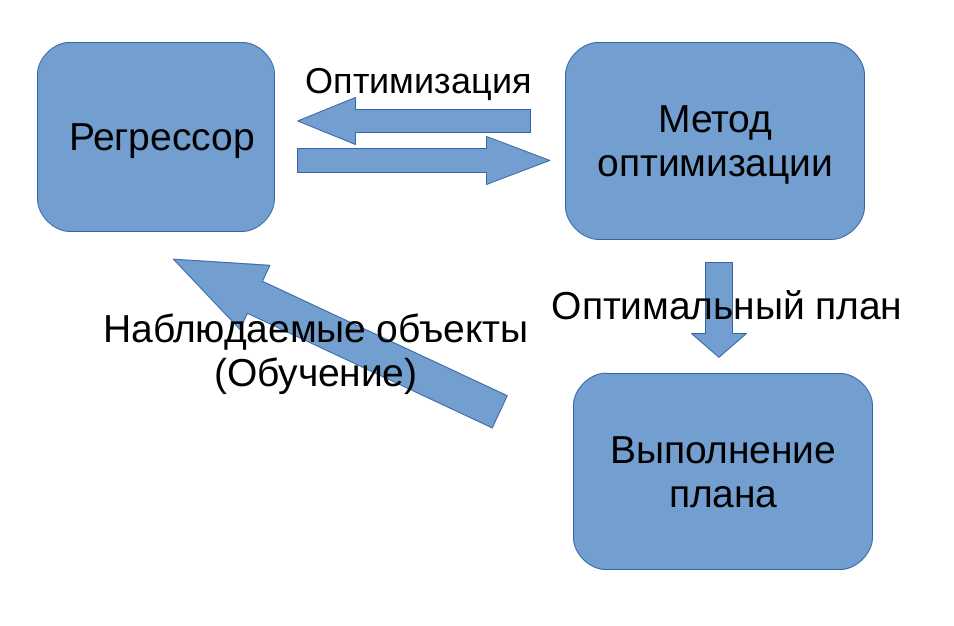
Let us explain the nature of the instability arising from the analytical solution. Our regressor responses are input to the optimizer, which is looking for the optimal plan. The objects we observe (executable plans) are the output values of the optimizer. Therefore, the objects we observe depend on the responses of the regressor. Such feedback systems are much more difficult to study than systems in which the regressor does not affect the environment. It is in these terms that the analytical solution by the Gauss method is unstable - it learns quickly, but offers more risky solutions, so the system as a whole works worse.

After a detailed study of the linear model, we found that it does not fully describe the data. Therefore, the best results from the methods we tested showed kNN.

kNN. A significant disadvantage of this method is the need to store in memory all objects, followed by the organization of a quick search for them. This situation can be significantly improved using the object selection algorithm. The idea of a naive object selection algorithm: if the prediction on an object is good enough, then it is not necessary to memorize this object.

This method is also more stable than linear regression: convergence on the TPC-H benchmark requires only 2 training cycles shown in the figure above.

What causes the use of machine learning

We present the results obtained for the kNN algorithm.


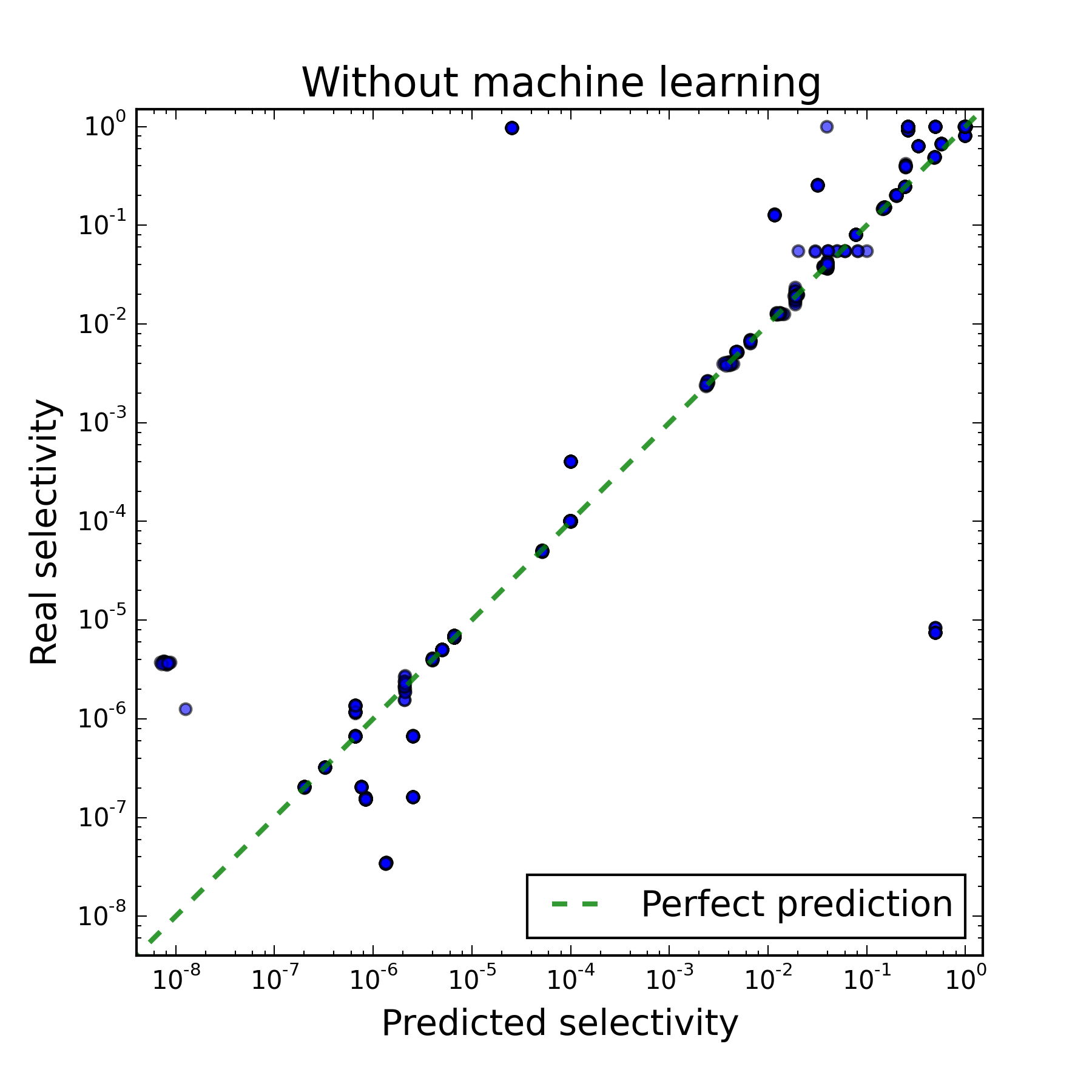Before machine learning	After machine learning

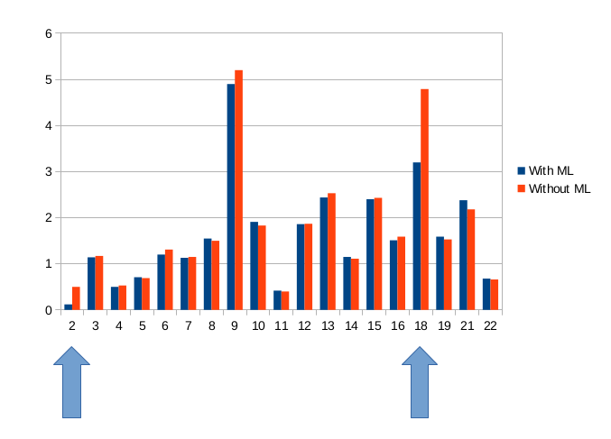
You can see that the proposed approach really speeds up the time for the DBMS. On one of the benchmark request types, the acceleration is 30-45%, on the other - 2-4 times.

What are the ways of development?

There are still many areas for further improvement of the existing prototype.

The problem of finding plans. The current algorithm ensures that in those plans to which the algorithm converges, the selectivity predictions will be correct. However, this does not guarantee the global optimality of the selected plans. The search for globally optimal plans or at least the best local optimum is a separate task.
Interrupt mode to stop the execution of an unsuccessful plan. In the standard PostgreSQL model, it does not make sense for us to interrupt the execution of the plan, since we have only one best plan and it does not change. With the introduction of machine learning, we can interrupt the implementation of the plan, in which serious mistakes were made in the prediction of selectivity, take into account the information received and choose a new best plan for implementation. In most cases, the new plan will differ significantly from the previous one.
Modes of obsolescence of information. During the operation of the DBMS, the data and typical queries change. Therefore, data that was obtained in the past may be irrelevant. Now our company is working on a good system for determining the relevance of information, and, accordingly, "forgetting" outdated information.

What was it?

In this article we:

dismantled the mechanism of the PostgreSQL scheduler;
noted problems in the current selectivity estimation algorithm;
showed how machine learning methods can be used to evaluate selectivity;
It was established experimentally that the use of machine learning leads to an improvement in the work of the scheduler and, accordingly, to an acceleration of the work of the DBMS.

Thanks for attention!