Non-local image smoothing algorithm
Removing noise from an image is one of the fundamental operations of computer vision. Smoothing algorithms are used almost everywhere: they can be both a stand-alone procedure for improving photos, and the first step for a more complex procedure, for example, for recognizing objects in an image. Therefore, there are a great many ways of smoothing, and I would like to tell you about one of them, which differs from the others by its good applicability on textures and images with a large number of identical details.
There are a lot of pictures under the cut, more accurate with traffic.
Briefly about the task. It is assumed that in some ideal world we can get the perfect image (matrix or vector
  elements), which ideally conveys information about the outside world. Unfortunately, we do not live in such a beautiful place, and therefore, for various reasons, we have to operate with images
  where
where  - matrix or noise vector. There are many models of noise, but in this article we will assume that - white Gaussian noise. According to the information we are trying to restore the image
  that will be as close as possible to the perfect image . Unfortunately, this is almost always impossible, since in case of noise some data is inevitably lost. In addition, the very formulation of the problem involves an infinite number of solutions.
As a rule, ordinary smoothing filters set a new value for each pixel using information about its neighbors. A cheap and angry Gaussian filter, for example, collapses an image matrix with a Gaussian matrix. As a result, in a new image, each pixel is a weighted sum of a pixel with the same number of the original image and its neighbors. A slightly different approach uses the median filter: it replaces each pixel with the median among all nearby pixels. The development of ideas for these methods of smoothing is a bilateral filter. This procedure takes a weighted sum around, relying both on the distance to the selected pixel and on the proximity of pixels in color.
')
However, all of the above filters use only information about nearby pixels. The main idea of a non-local smoothing filter is to use all the information in the image, and not just the pixels adjacent to the one being processed. How does this work, because often the values at remote points do not depend on each other?
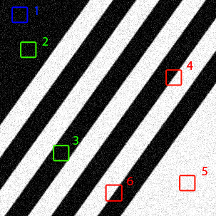
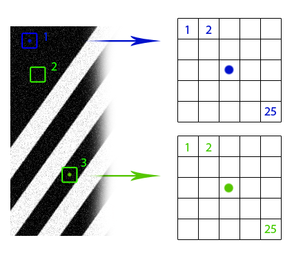
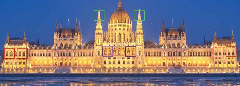
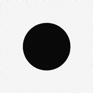
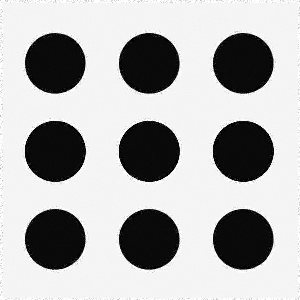
It is obvious that if we have several images of the same object with different noise levels, then we can compose them into one image without noise. If these several objects are placed in different places of the same image, then we can still use this additional information (the small thing is to first find these objects). And even if these objects look a bit different or partially overlapped, we still have redundant data that can be used. The non-local smoothing filter uses this idea: it finds similar areas of the image and applies the information from them for mutual averaging. Of course, that parts of the image are similar, does not mean that they belong to the same objects, but, as a rule, the approximation is quite good. Look at the drawing with lines. Obviously, windows 2 and 3 are similar to window 1, but windows 4, 5 and 6 are not. In the photo of the Hungarian Parliament, you can also notice a large number of identical elements.
Suppose that if a neighborhood of a pixel in one window looks like a neighborhood of the corresponding pixel in another window, then the values of these pixels can be used for mutual averaging (blue and green points in the figure). But how to find these similar windows? How to match their weights, with what force do they influence each other? We formalize the concept of "similarity" of image pieces. First, we need the function of distinguishing two pixels. Everything is simple here: for black-and-white images, the modulus of the difference in pixel values is usually used. If there is any additional information about the image, options are possible. For example, if it is known that a clean image consists of objects of absolutely black color on a completely white background, a good idea would be to use a metric that matches the zero distance to pixels that are not very different in color. In the case of color images, again, options are possible. You can use the Euclidean metric in RGB format or something more cunning in HSV format. The “differentness” of the image windows is just the sum of the differences in their pixels.
Now it would be good to convert the resulting value to a more familiar weight format.![w \ in [0, 1]](http://tex.s2cms.ru/svg/w%20%5Cin%20%5B0%2C%201%5D) . Let's transfer the difference of windows calculated at the previous step into some decreasing (or at least non-increasing) function and normalize the result obtained by sum of the values of this function on all possible windows. Usually, the role of such a function appears familiar to all the tooth gnash
. Let's transfer the difference of windows calculated at the previous step into some decreasing (or at least non-increasing) function and normalize the result obtained by sum of the values of this function on all possible windows. Usually, the role of such a function appears familiar to all the tooth gnash  where
where  - distance, and
  - parameter of scatter of scales. The more the less effect the difference between the windows on anti-aliasing. With
  , all windows regardless of the difference between them equally contribute to each pixel, and the image will turn out perfectly gray, with
  , significant weight will be only at the window corresponding to itself, and smoothing will not work.
Thus, a naive mathematical model of a non-local averaging filter looks like this:
%20%3D%20%5Csum_%7Bj%20%5Cin%20I%7Dw(i%2C%20j)I(j))
 -th pixel of the resulting image is equal to the sum of all pixels of the original image, taken with weights
  where weight is
%20%3D%20%5Cfrac%7B1%7D%7BZ(i)%7De%5E%7B-%5Cfrac%7B%5C%7CI(N_i)%20-%20I(N_j)%5C%7C%5E2_2%7D%7Bh%5E2%7D%7D)
and the normalizing divider
%20%3D%20%5Csum_%7Bj%20%5Cin%20I%7De%5E%7B-%5Cfrac%7B%5C%7CI(N_i)%20-%20I(N_j)%5C%7C%5E2_2%7D%7Bh%5E2%7D%7D)
Alternative metrics suggested above:
%3D%5Cbegin%7Bcases%7D%0A%20%20%20%200%2C%20%26%20%5Ctext%7Bif%20%24%7Cx-y%7C%3Ct%24%7D.%5C%5C%0A%20%20%20%20%7Cx-y%7C-t%20%2C%20%26%20%5Ctext%7Botherwise%7D.%0A%20%20%5Cend%7Bcases%7D%0A)
In all cases%20-%20I(N_j)%5C%7C) denotes the element by element difference between the windows, as described above.
denotes the element by element difference between the windows, as described above.
If you look closely, the final formula is almost the same as that of the bilateral filter, only in the exponent instead of the geometric distance between the pixels and the color difference there is a difference between the image patches and the summation is carried out over all pixels of the image.
Obviously, the complexity of the proposed algorithm)) where
where  - the radius of the window, which is used to calculate the similarity of parts of the image, and - the total number of pixels, because for each pixel we compare its size neighborhood
  with a neighborhood of every other pixel. This is not too good, because the naive implementation of the algorithm is slow enough even in 300x300 images. The following improvements are usually suggested:
A common question that arises when considering this algorithm is: why do we use only the values of the central pixel in the area? Generally speaking, nothing prevents you from summing over the entire domain in the basic formula, as in bilateral anti-aliasing, and this even slightly affects the complexity, but the result of the modified algorithm is likely to be too vague. Do not forget that in real images even identical objects are rarely absolutely identical, and such a modification of the algorithm will average them. To use information from adjacent image elements, you can pre-perform the usual bilateral anti-aliasing. Although if it is known that the original objects were or should end up being exactly the same (text smoothing), then such a change would be beneficial.
Naive implementation of the algorithm (C + OpenCV 2.4.11):
Let's look at some results:
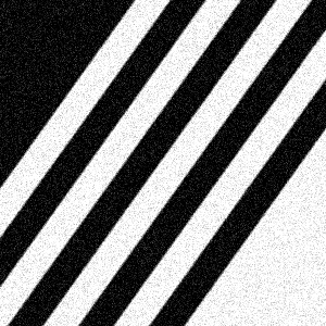

Note the near perfect smoothing and the sharp edges of the lines. The more identical square areas in the image, the better the algorithm works. Here the program had enough examples for each type of neighborhood, because all the square areas along the lines are about the same.
Of course, everything is not so rosy for those cases where the "similarity" of areas cannot be detected by a simple square window. For example:

Although the background and the inside of the circle smoothed out well, artifacts remained along the circumference. Of course, the algorithm cannot understand that the right side of the circle is the same as the left, only rotated 180 degrees, and use this when smoothing. Such an obvious blunder can be corrected by viewing rotated windows, but then the execution time will increase by as many times as the window turns are considered.
So that there is no doubt that the algorithm can smooth not only straight lines, here is another example that at the same time illustrates the importance of choosing a smoothing parameter:


In the second image, we see approximately the same artifacts as in the previous case. It's not a lack of similar windows, but a parameter that is too small. : even similar areas gain too low weights. In the fourth picture, on the contrary, was chosen too large , and all areas received roughly the same weight. The third represents the middle ground.
Another example of the work on the text. Even a small and very noisy image is processed well enough for subsequent use by the machine (after equalization of the histogram and focusing, of course):
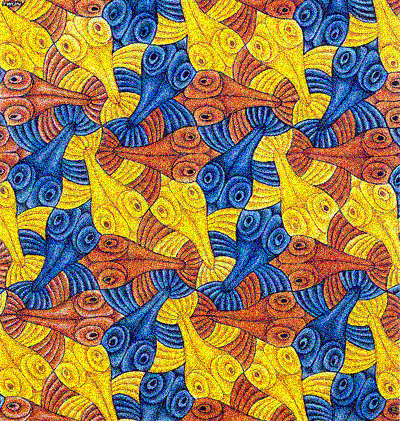
A few more examples from the site where you can apply an already optimized non-local smoothing algorithm:
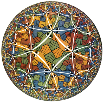

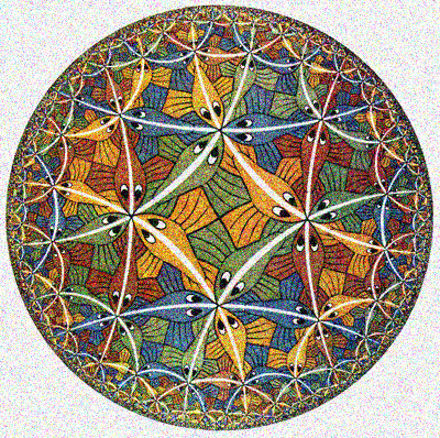

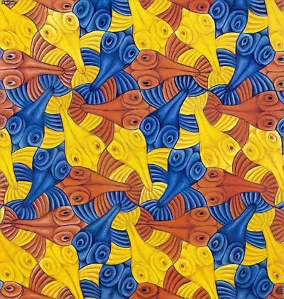
Order: original, noisy, restored. Notice how well Escher’s drawings were cleaned up with many similar elements. Only black lines became more transparent and smoothed texture.
Unfortunately, the high computational complexity of the algorithm limits its application in practice, however, it shows good results on the tasks of smoothing images with repeating elements. The main problem of this algorithm lies in its main idea of calculating weights. It is necessary for each pixel to go through the surroundings of all other pixels. Even if we assume that double viewing of all pixels is an inevitable evil, then viewing of its neighbors seems superfluous, because even for a window radius of 3, it increases the time for calculating weights by 49 times. Let's go back a little to the original idea. We want to find similar places in the image to use to smooth each other out. But we don’t have to compare all possible windows in the image pixel by pixel to find similar places. We already have a good way to identify and compare interesting image elements! Of course, I'm talking about a variety of feature descriptors. Usually, this means SIFT, but in our case it is better to use something less accurate, because the goal at this stage is to find many quite similar areas, and not several exactly the same. In the case of the use of descriptors, the step of calculating the scales is as follows:
The advantages of this approach:
Disadvantages:
Findings:
Thus, we have considered a smoothing algorithm that uses information about similar objects in the image to best approximate a clean image. From such a “pseudo-recognition”, the transition to a real smoothing is not far after the selection of similar objects. Indeed, modern approaches to image restoration use neural networks for this purpose and, as a rule, they actually do better and faster. However, neural networks require more skill in programming and fine tuning. Even such an algorithm, which only simulates recognition, can give a comparable and sometimes better result.
Antoni Buades, Bartomeu Coll A Non-local Algorithm For Image Denoising
Yifei Lou, Paolo Favaro, Stefano Soatto, and Andrea Bertozzi Nonlocal Similarity Image Filtering
There are a lot of pictures under the cut, more accurate with traffic.
Preliminary information
Briefly about the task. It is assumed that in some ideal world we can get the perfect image
As a rule, ordinary smoothing filters set a new value for each pixel using information about its neighbors. A cheap and angry Gaussian filter, for example, collapses an image matrix with a Gaussian matrix. As a result, in a new image, each pixel is a weighted sum of a pixel with the same number of the original image and its neighbors. A slightly different approach uses the median filter: it replaces each pixel with the median among all nearby pixels. The development of ideas for these methods of smoothing is a bilateral filter. This procedure takes a weighted sum around, relying both on the distance to the selected pixel and on the proximity of pixels in color.
')
Filter idea
However, all of the above filters use only information about nearby pixels. The main idea of a non-local smoothing filter is to use all the information in the image, and not just the pixels adjacent to the one being processed. How does this work, because often the values at remote points do not depend on each other?
It is obvious that if we have several images of the same object with different noise levels, then we can compose them into one image without noise. If these several objects are placed in different places of the same image, then we can still use this additional information (the small thing is to first find these objects). And even if these objects look a bit different or partially overlapped, we still have redundant data that can be used. The non-local smoothing filter uses this idea: it finds similar areas of the image and applies the information from them for mutual averaging. Of course, that parts of the image are similar, does not mean that they belong to the same objects, but, as a rule, the approximation is quite good. Look at the drawing with lines. Obviously, windows 2 and 3 are similar to window 1, but windows 4, 5 and 6 are not. In the photo of the Hungarian Parliament, you can also notice a large number of identical elements.
Suppose that if a neighborhood of a pixel in one window looks like a neighborhood of the corresponding pixel in another window, then the values of these pixels can be used for mutual averaging (blue and green points in the figure). But how to find these similar windows? How to match their weights, with what force do they influence each other? We formalize the concept of "similarity" of image pieces. First, we need the function of distinguishing two pixels. Everything is simple here: for black-and-white images, the modulus of the difference in pixel values is usually used. If there is any additional information about the image, options are possible. For example, if it is known that a clean image consists of objects of absolutely black color on a completely white background, a good idea would be to use a metric that matches the zero distance to pixels that are not very different in color. In the case of color images, again, options are possible. You can use the Euclidean metric in RGB format or something more cunning in HSV format. The “differentness” of the image windows is just the sum of the differences in their pixels.
Now it would be good to convert the resulting value to a more familiar weight format.
Thus, a naive mathematical model of a non-local averaging filter looks like this:
and the normalizing divider
Alternative metrics suggested above:
In all cases
If you look closely, the final formula is almost the same as that of the bilateral filter, only in the exponent instead of the geometric distance between the pixels and the color difference there is a difference between the image patches and the summation is carried out over all pixels of the image.
Efficiency considerations and implementation
Obviously, the complexity of the proposed algorithm
- Obviously, it is not necessary to count all the weights all the time, because the pixel weight
and vice versa - are equal. If you save the calculated weight, the execution time is halved, but it takes
memory for storing weights.
- For most real-world images, the weights between most of the pixels will be zero. So why not zero them at all? You can use heuristics based on image segmentation, which will suggest where to count the weight pixel by pixel meaningless.
- When calculating weights, an exhibitor can be replaced by a function that is cheaper to calculate. At least piecewise interpolation of the same exponent.
A common question that arises when considering this algorithm is: why do we use only the values of the central pixel in the area? Generally speaking, nothing prevents you from summing over the entire domain in the basic formula, as in bilateral anti-aliasing, and this even slightly affects the complexity, but the result of the modified algorithm is likely to be too vague. Do not forget that in real images even identical objects are rarely absolutely identical, and such a modification of the algorithm will average them. To use information from adjacent image elements, you can pre-perform the usual bilateral anti-aliasing. Although if it is known that the original objects were or should end up being exactly the same (text smoothing), then such a change would be beneficial.
Naive implementation of the algorithm (C + OpenCV 2.4.11):
#include "targetver.h" #include <stdio.h> #include <math.h> #include <opencv2/opencv.hpp> #include "opencv2/imgproc/imgproc.hpp" #include "opencv2/imgproc/imgproc_c.h" #include "opencv2/highgui/highgui.hpp" #include "opencv2/core/core.hpp" #include "opencv2/features2d/features2d.hpp" #include "opencv2/calib3d/calib3d.hpp" #include "opencv2/nonfree/nonfree.hpp" #include "opencv2/contrib/contrib.hpp" #include <opencv2/legacy/legacy.hpp> #include <stdlib.h> #include <stdio.h> using namespace cv; /* Returns measure of diversity between two pixels. The more pixels are different the bigger output number. Usually it's a good idea to use Euclidean distance but there are variations. */ double distance_squared(unsigned char x, unsigned char y) { unsigned char zmax = max(x, y); unsigned char zmin = min(x, y); return (zmax - zmin)*(zmax - zmin); } /* Returns weight of interaction between regions: the more dissimilar are regions the less resulting influence. Usually decaying exponent is used here. If distance is Euclidean, being combined, they form a typical Gaussian function. */ double decay_function(double x, double dispersion) { return exp(-x/dispersion); } int conform_8bit(double x) { if (x < 0) return 0; else if (x > 255) return 255; else return static_cast<int>(x); } double distance_over_neighbourhood(unsigned char* data, int x00, int y00, int x01, int y01, int radius, int step) { double dispersion = 15000.0; //should be manually adjusted double accumulator = 0; for(int x = -radius; x < radius + 1; ++x) { for(int y = -radius; y < radius + 1; ++y) { accumulator += distance_squared(static_cast<unsigned char>(data[(y00 + y)*step + x00 + x]), static_cast<unsigned char>(data[(y01 + y)*step + x01 + x])); } } return decay_function(accumulator, dispersion); } int main(int argc, char* argv[]) { int similarity_window_radius = 3; //may vary; 2 is enough for text filtering char* imageName = "text_noised_30.png"; IplImage* image = 0; image = cvLoadImage(imageName, CV_LOAD_IMAGE_GRAYSCALE); if (image == NULL) { printf("Can not load image\n"); getchar(); exit(-1); } CvSize currentSize = cvGetSize(image); int width = currentSize.width; int height = currentSize.height; int step = image->widthStep; unsigned char *data = reinterpret_cast<unsigned char *>(image->imageData); vector<double> processed_data(width*height, 0); //External cycle for(int x = similarity_window_radius + 1; x < width - similarity_window_radius - 1; ++x) { printf("x: %d/%d\n", x, width - similarity_window_radius - 1); for(int y = similarity_window_radius + 1; y < height - similarity_window_radius - 1; ++y) { //Inner cycle: computing weight map vector<double> weight_map(width*height, 0); double* weight_data = &weight_map[0]; double norm = 0; for(int xx = similarity_window_radius + 1; xx < width - similarity_window_radius - 1; ++xx) for(int yy = similarity_window_radius + 1; yy < height - similarity_window_radius - 1; ++yy) { double weight = distance_over_neighbourhood(data, x, y, xx, yy, similarity_window_radius, step); norm += weight; weight_map[yy*step + xx] = weight; } //After all weights are known, one can compute new value in pixel for(int xx = similarity_window_radius + 1; xx < width - similarity_window_radius - 1; ++xx) for(int yy = similarity_window_radius + 1; yy < height - similarity_window_radius - 1; ++yy) processed_data[y*step + x] += data[yy*step + xx]*weight_map[yy*step + xx]/norm; } } //Transferring data from buffer to original image for(int x = similarity_window_radius + 1; x < width - similarity_window_radius - 1; ++x) for(int y = similarity_window_radius + 1; y < height - similarity_window_radius - 1; ++y) data[y*step + x] = conform_8bit(processed_data[y*step + x]); cvSaveImage("gray_denoised.png", image); cvReleaseImage(&image); return 0; } Examples
Let's look at some results:
Note the near perfect smoothing and the sharp edges of the lines. The more identical square areas in the image, the better the algorithm works. Here the program had enough examples for each type of neighborhood, because all the square areas along the lines are about the same.
Of course, everything is not so rosy for those cases where the "similarity" of areas cannot be detected by a simple square window. For example:
Although the background and the inside of the circle smoothed out well, artifacts remained along the circumference. Of course, the algorithm cannot understand that the right side of the circle is the same as the left, only rotated 180 degrees, and use this when smoothing. Such an obvious blunder can be corrected by viewing rotated windows, but then the execution time will increase by as many times as the window turns are considered.
So that there is no doubt that the algorithm can smooth not only straight lines, here is another example that at the same time illustrates the importance of choosing a smoothing parameter:
In the second image, we see approximately the same artifacts as in the previous case. It's not a lack of similar windows, but a parameter that is too small.
Another example of the work on the text. Even a small and very noisy image is processed well enough for subsequent use by the machine (after equalization of the histogram and focusing, of course):
A few more examples from the site where you can apply an already optimized non-local smoothing algorithm:
Order: original, noisy, restored. Notice how well Escher’s drawings were cleaned up with many similar elements. Only black lines became more transparent and smoothed texture.
Scaling with descriptor points
Unfortunately, the high computational complexity of the algorithm limits its application in practice, however, it shows good results on the tasks of smoothing images with repeating elements. The main problem of this algorithm lies in its main idea of calculating weights. It is necessary for each pixel to go through the surroundings of all other pixels. Even if we assume that double viewing of all pixels is an inevitable evil, then viewing of its neighbors seems superfluous, because even for a window radius of 3, it increases the time for calculating weights by 49 times. Let's go back a little to the original idea. We want to find similar places in the image to use to smooth each other out. But we don’t have to compare all possible windows in the image pixel by pixel to find similar places. We already have a good way to identify and compare interesting image elements! Of course, I'm talking about a variety of feature descriptors. Usually, this means SIFT, but in our case it is better to use something less accurate, because the goal at this stage is to find many quite similar areas, and not several exactly the same. In the case of the use of descriptors, the step of calculating the scales is as follows:
- Pre-count the descriptors at each point of the image.
- We pass through the image and for each pixel
- o Pass by every other pixel
- o Compare descriptors
- o If descriptors are similar, then compare windows pixel by pixel and count the weight
- o If different, reset weight
- In order not to pass through the image a second time, the calculated weights and coordinates of the pixels are entered into a separate list. When the list has accumulated a sufficient number of items, you can stop the search.
- If you did not manage to find the specified number of similar points (the pixel is not noticeable), simply go through the image and count the weights as usual
The advantages of this approach:
- Smoothing is improved at specific points that are usually most interesting to us.
- If the image has many similar special points, the speed increase is noticeable.
Disadvantages:
- Not the fact that there will be many similar points to recoup the counting of descriptors.
- The result and acceleration of the algorithm strongly depend on the choice of the descriptor.
Conclusion
Findings:
- The algorithm works well on periodic textures.
- The algorithm smooths homogeneous areas well.
- The larger the image, the more similar areas and the better the algorithm works. But godlessly long.
- Areas for which it was not possible to find such ones are poorly smoothed out (solved by preliminary use of a bilateral filter or by examining turns of windows)
- As with many other algorithms, it is necessary to adjust the value of the smoothing parameter.
Thus, we have considered a smoothing algorithm that uses information about similar objects in the image to best approximate a clean image. From such a “pseudo-recognition”, the transition to a real smoothing is not far after the selection of similar objects. Indeed, modern approaches to image restoration use neural networks for this purpose and, as a rule, they actually do better and faster. However, neural networks require more skill in programming and fine tuning. Even such an algorithm, which only simulates recognition, can give a comparable and sometimes better result.
Sources
Antoni Buades, Bartomeu Coll A Non-local Algorithm For Image Denoising
Yifei Lou, Paolo Favaro, Stefano Soatto, and Andrea Bertozzi Nonlocal Similarity Image Filtering
Source: https://habr.com/ru/post/273159/
All Articles