Covering graphs in software testing, part 2

Most programs and algorithms can be represented as a graph consisting of a set of vertices ( N ) and edges ( E ). Coverage of graphs in testing is useful because you can design tests using different coverage criteria and identify errors. With regard to testing the black box, then covering graphs here can also be of great importance if you have to work with states and transitions, entity state graphs, etc. If the graph is rather complicated, different coverage criteria will allow assessing the sufficiency of the test suite.

In the first part : definitions, covering vertices, edges, paths, cyclomatic complexity.

Definitions: basic paths

• A simple path is a path where no vertex appears more than once, except the initial and final one (which may coincide). Simple paths do not have internal loops. A simple path of maximum length is called the main one.
• The main path is a simple path that is not a segment of any other simple path. Let us rephrase for clarity: the main path has no internal cycles (the vertices are unique), and it is the longest among similar paths. If it can be made longer, then it is a segment of another simple path, which means it will not be the main one. (It turns out this is a very simple concept as soon as you become aware of it.)
• For example, consider the path [1, 2, 3, 4, 5, 6, 1] (not related to any of the graphs in this article). This is a simple path, since all its vertices are unique, except the first and last. Based on the assumption that this path is not a segment of any other, it will also be the main one. On the other hand, the path [1, 2, 3, 4] can in no way be the main one, since we know that there are [1, 2, 3, 4, 5, 6, 1], and [1, 2, 3, 4] is definitely its segment. And that means not the main one.
• A closed path is a basic path of nonzero length that begins and ends at the same vertex. [1, 2, 3, 4, 5, 6, 1] - a simple way, which is also the main and closed.

Covering main paths (POP)

Requirements for test coverage contain all the major paths in column G.

There are fewer simple paths in the graph than the main ones. Therefore, covering all the main paths in a graph is a good way to reduce the total number of paths that should be considered. The number of test paths is reduced without the need to rely on the tester's subjective judgments, as in covering the specified paths, and the requirements will not be computationally laborious, as in full coverage of the paths.
')
The approach is simple: define a set of basic paths and prepare test cases that implement each of them.

Covering the main paths includes covering tops, edges and paired covering of edges. According to some sources, POP does not include paired finning. The following arguments are given: if there is an edge at the vertex n that extends from it and is included in it, this will create the following requirement for pairwise covering the edges: [n, n, m], where m is the receiver n . Since [n, n, m] is obviously not the main path, the cover of the main paths cannot contain this path, which in turn means that the cover of the main paths does not include the pairwise covering of the ribs. This logic is not entirely correct, since the test requirements for paired edge coverage include not [n, n, m], but [n, n], which, in turn, is an absolutely correct basic path.

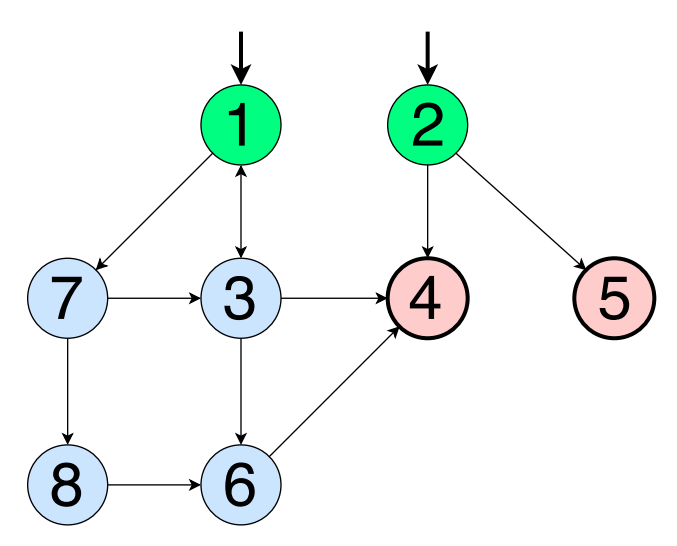
requirements = {
[1, 2, 6],
[1, 2, 3, 4, 6],
[1, 2, 3, 4, 5],
[2, 3, 4, 5, 2],
[3, 4, 5, 2, 3],
[4, 5, 2, 3, 4],
[5, 2, 3, 4, 5],
}
path (t) = {
[1, 2, 6],
[1, 2, 3, 4, 6],
[1, 2, 3, 4, 5, 2, 3, 4, 5, 2, 6]
}

The reason why the last test path is somewhat longer is as follows: we need to go through the cycle not once but twice to cover all the requirements.

Search for main paths

In order to cover the main paths, you must first find them all. The easiest way to do this is to start by listing the longest paths in the graph.



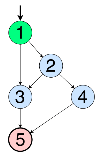
Using the graph from the example above, we begin by listing the longest paths.

[1, 2, 3, 5]
[1, 2, 4, 5]

By definition, a main path is a simple path that is not a segment of another path. In general, in the graph there are basic paths shorter than the longest. These paths are “hidden” within the cycles (details below), but in the case of the graph above, the last main path is a straight line [1, 3, 5]. All other paths, for example, [2, 3, 5], are segments of the paths already listed. A complete set of basic paths is as follows:

[1, 2, 3, 5]
[1, 2, 4, 5]
[1, 3, 5]

As mentioned above, the main paths “hide” inside the cycles. If there are x vertices in the loop, there will be x additional main paths.



If we used the method that was used before, we would get the following basic ways:

[1, 2, 3, 4, 6]
[1, 2, 6]
[1, 2, 3, 4, 5]

Starting from vertex 2, we go around the loop once and return to vertex 2. This is the first main path. Starting at vertex 3, we go around the loop again, returning to it. This is the second main way. If we repeat the same for vertices 4 and 5, we get 4 additional basic paths. Compare them with those already listed above, and you will see that these are completely new basic paths (that is, they are not segments of any of the above). The main paths that begin and end at the same vertex are called closed.

[2, 3, 4, 5, 2]
[3, 4, 5, 2, 3]
[4, 5, 2, 3, 4]
[5, 2, 3, 4, 5]

Now that we have become acquainted with the main and closed paths, we can talk about some more criteria.

Simple Closed Path Coverage

The requirements for an SDPR contain at least one closed path for any reachable vertex in G that starts and ends a closed path.

Simply put, this means that among all the closed paths listed above, we take one for each cycle. If there is one more cycle in the graph, we will need to take another closed path that covers the vertices of this cycle in order to satisfy the conditions of the OOP.

As an example, consider again the graph from the previous section.

requirements = {[2, 3, 4, 5, 2]}
path (T) = {[1, 2, 3, 4, 5, 2, 6]}

An SDPR requires only one closed path for each cycle if all vertices in all closed paths are covered.

Full coverage closed paths (LARP)

Similar to the SDPR, but includes all closed paths.

Requirements contain all closed paths for each reachable vertex in the graph.

requirements = {
[2, 3, 4, 5, 2],
[3, 4, 5, 2, 3],
[4, 5, 2, 3, 4],
[5, 2, 3, 4, 5]
}
path (t) = {
[1, 2, 3, 4, 5, 2, 3, 4, 5, 2, 6]
}

We have included all closed paths in the coverage, as required by the LARP. If you have not yet noticed, it is important to realize that the LARP and LARE have a strange property to skip vertices and edges of the graph that are not included in closed paths. This means that they do not include paired edge finishes, edge finishes or vertex finishes. Look at the illustration of the inclusions below.