Neural network in Python, part 2: gradient descent
Part 1
In the first part, I described the basic principles of reverse propagation in a simple neural network. The network allowed us to measure how each of the weights of the network contributes to the error. And it allowed us to change weights with the help of another algorithm - gradient descent.
The essence of what is happening is that back distribution does not bring optimization to the network. It moves the wrong information from the end of the network to all the weights inside, so that another algorithm can already optimize these weights so that they match our data. But in principle, we have in abundance other methods of nonlinear optimization that we can use with back propagation:
Some optimization methods:
')
Difference visualization:
Different methods are suitable for different cases, and in some cases can even be combined. In this lesson we will look at gradient descent - this is one of the simplest and most popular algorithms for optimizing neural networks. Thus, we will improve our neural network through settings and parameterization.
Suppose you have a red ball in a round basket (picture below). The ball is trying to find the bottom. This is an optimization. In our case, the ball optimizes its position, from left to right, in search of the lowest point in the bucket.
The ball has two options for movement - left or right. The goal is to take a position as low as possible. If you were to control the ball from the keyboard, you would need to press the buttons left and right.
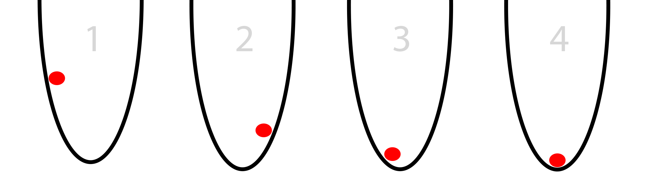
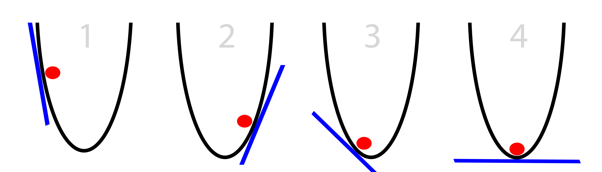
In our case, the ball knows only the slope of the bucket's side at its current position (tangent to the wall, shown in blue). Note that if the bias is negative, the ball needs to move to the right. If positive, left. Obviously, this information is quite enough to find the bottom of the bucket in several iterations. This kind of optimization is called gradient optimization.
The simplest case of the HS:
The question is how far the ball should move at each step. From the picture it is clear that the farther it is from the bottom, the steeper the slope. We will improve the algorithm using this knowledge. Also assume that the bucket is located on the plane (x, y). Therefore, the position of the ball is determined by the x coordinate. Increasing x causes the ball to move to the right.
The simplest gradient descent:
This algorithm is already slightly optimized, because in case of a large slope we make significant shifts, and for small slopes we make a small shift. As a result, when approaching the bottom of the basket, the ball makes ever-smaller oscillations until it reaches a point with a zero incline. This will be a convergence point.
Gradient descent is imperfect. Consider his problems and how people get around them.
Our step depends on the size of the slope. If it is too big, we can jump over the point we need. If we do not jump it very much, it is not scary. But you can jump it so hard that we will be even further away from it than we were before.
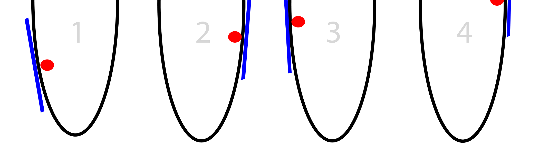
And already there, naturally, we will find an even greater bias, jump even further, and obtain divergence.
Simply multiply them by a number from 0 to 1 (for example, 0.01). Let's call this constant alpha. After such a cast, our network will converge, because we no longer jump the desired point so much.
Improved gradient descent:
alpha = 0.1 (or any number from 0 to 1)
Sometimes a bucket has a very tricky shape, and simply following a slope will not lead you to the absolute minimum.
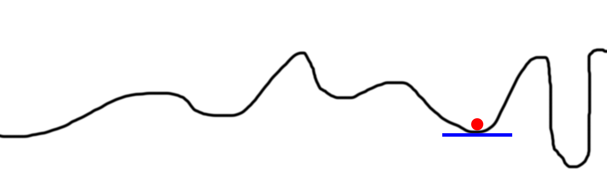
This is the most difficult problem of gradient descent. There are many ways to circumvent it. Usually they use a random search, trying different parts of the bucket.
Well, but if we use chance to search for a global minimum, why should we be optimizing at all? Maybe we will look for a solution at random?
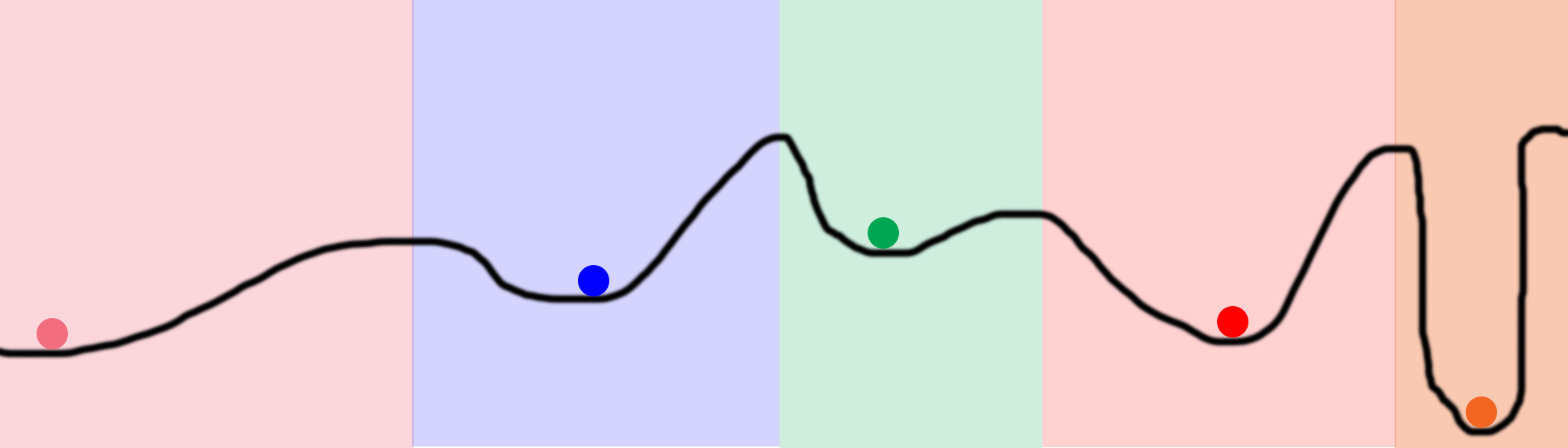
Consider this chart. Suppose we placed 100 balls on the line and began to optimize them. As a result, they will be in 5 positions marked with colored circles. Colored areas indicate the ownership of each local minimum. For example, if the ball enters the blue area, it will end up in the blue minimum. That is, to explore the entire space, we need to accidentally find only 5 places. This is much better than a completely random search that tries every place on the line.
Regarding neural networks, this can be achieved by setting very large hidden levels. Each hidden node in the level starts working in its random state. Then each node converges to some final state. Their size may allow a network user to try thousands, or millions, of different local minima on the same network.
Note 1: these neural networks are also profitable. They have the opportunity to search the space without calculating it entirely. We can search the entire black line in the figure above using only 5 balls and a small number of iterations. Search by brute force would require several orders of magnitude more processor power.
Note 2: an inquisitive reader will ask: “Why should we allow a bunch of different nodes to converge to the same point? This is a waste of computing power! ". Good question. There are some approaches that avoid hidden nodes - these are Dropout and Drop-Connect, which I am going to describe later.
Problem 3: slopes too small
Sometimes biases are too small. Consider this schedule.
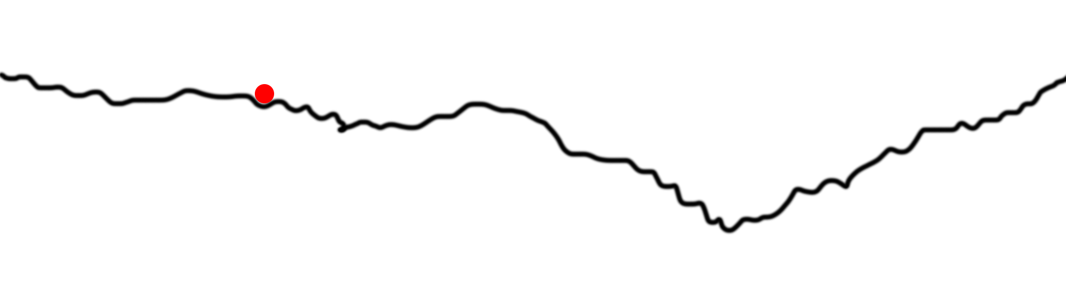
Our ball is stuck. This will happen if alpha is too small. He immediately finds a local minimum and ignores everything else. And, of course, with such small movements, convergence will take a very long time.

Obviously, you can increase the alpha, and even multiply our deltas by a number greater than 1. It is rarely used, but it happens.
So how are these balls and lines connected to neural networks and back distribution? This topic is as important as it is complex.
In the neural network, we try to minimize errors with respect to weights. The line represents a network error relative to the position of one of the weights. If we calculated the network error for any possible value of one of the weights, the result would be represented by such a line. Then we would choose the weight value corresponding to the smallest error (the lowest part of the curve). I say - one weight, since our graph is two-dimensional. x is the value of weight, and y is the error of the neural network at the moment when the weight is in the value of x.
Now let's look at how this process works in a simple two-level neural network.
In our case there will be one error on the output, counted in line 35 (layer_1_error = layer_1 - y). Since we have 2 weights, the graph with errors will be located in three-dimensional space. This will be the space (x, y, z) where errors are vertically, and x and y are weights in syn0.
Let's try to draw the error surface for our data set. How do we calculate the error for a given set of weights? This calculation is in lines 31, 32 and 35:
If we draw a general error for any set of weights (from -10 to 10 for x and y), we get something like this:
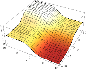
In fact, everything is simple - we count all possible combinations of weights, and the error generated by the network on each of the sets. x is the first weight of synapse_0, and y is the second weight of synapse_0. z is an error. As you can see, the output is positively correlated with the first input set. Therefore, the error is minimal when x is large. What about u? When is it optimal?
So, if the indicated 3 lines calculate the error, then the following optimize the network to reduce it. Here is the gradient descent.
Recall our pseudocode:
This is it. The only change is that we optimize 2 weights, not just one. The logic is the same.
What is alpha? As described above, this parameter reduces the size of each iterative update. At the last moment, before updating the scales, we multiply the size of the update by alpha (usually between 0 and 1). And such a minimal change in the code greatly affects its ability to train.
Let's return to our three-level network from the previous article and add the alpha parameter to the right place. Then we will conduct experiments to bring all our ideas about alpha into correspondence with the real code.
What conclusions can be drawn from different alpha values?
Alpha = 0.001
With a very low value, the network does not converge at all. Scale updates are too small. Little has changed even after 60,000 iterations. This is our problem number 3: when the slopes are too small.
Alpha = 0.01
A good convergence, smoothly held over 60,000 repetitions, but still did not converge as close to the goal as other cases. The same problem number 3.
Alpha = 0.1
At first, they went pretty quickly, but then they slowed down. This is still the 3rd problem.
Alpha = 1
An inquisitive reader will notice that the convergence in this case is exactly the same as if there were no alpha. We multiply by 1.
Alpha = 10
Surprise - alpha more than one unit led to the achievement of the result of just 10,000 repetitions. So, our update weights before this was too small. So the weights were moving in the right direction, just before that they were moving too slowly.
Alpha = 100
Too large values are counterproductive. The network steps are so large that it cannot find the lowest point on the surface of errors. This is our problem number 1. The network just jumps back and forth over the surface of errors and nowhere finds the minimum.
Alpha = 1000
The error increases instead of decreasing, and it stops at a value of 0.5. This is a more extreme version of problem number 3.
Consider the results closer.
In the code above, I count the number of times the derivative changes direction. This corresponds to the “Update Direction Changes” output. If the bias (derivative) changes direction, then we have passed over the local minimum and we need to return. , , , .
:
, . .
32 — 0.0009, 4 – 0.0013. This is quite important. 3 . , , . , .
Let's get the code right away!
import numpy as np X = np.array([ [0,0,1],[0,1,1],[1,0,1],[1,1,1] ]) y = np.array([[0,1,1,0]]).T alpha,hidden_dim = (0.5,4) synapse_0 = 2*np.random.random((3,hidden_dim)) - 1 synapse_1 = 2*np.random.random((hidden_dim,1)) - 1 for j in xrange(60000): layer_1 = 1/(1+np.exp(-(np.dot(X,synapse_0)))) layer_2 = 1/(1+np.exp(-(np.dot(layer_1,synapse_1)))) layer_2_delta = (layer_2 - y)*(layer_2*(1-layer_2)) layer_1_delta = layer_2_delta.dot(synapse_1.T) * (layer_1 * (1-layer_1)) synapse_1 -= (alpha * layer_1.T.dot(layer_2_delta)) synapse_0 -= (alpha * XTdot(layer_1_delta)) Part 1: Optimization
In the first part, I described the basic principles of reverse propagation in a simple neural network. The network allowed us to measure how each of the weights of the network contributes to the error. And it allowed us to change weights with the help of another algorithm - gradient descent.
The essence of what is happening is that back distribution does not bring optimization to the network. It moves the wrong information from the end of the network to all the weights inside, so that another algorithm can already optimize these weights so that they match our data. But in principle, we have in abundance other methods of nonlinear optimization that we can use with back propagation:
Some optimization methods:
- Annealing
- Stochastic gradient descent
- AW-SGD (new!)
- Momentum (SGD)
- Nesterov Momentum (SGD)
- AdaGrad
- Adadelta
- ADAM
- Bfgs
- Lbfgs
')
Difference visualization:
Different methods are suitable for different cases, and in some cases can even be combined. In this lesson we will look at gradient descent - this is one of the simplest and most popular algorithms for optimizing neural networks. Thus, we will improve our neural network through settings and parameterization.
Part 2: Gradient Descent
Suppose you have a red ball in a round basket (picture below). The ball is trying to find the bottom. This is an optimization. In our case, the ball optimizes its position, from left to right, in search of the lowest point in the bucket.
The ball has two options for movement - left or right. The goal is to take a position as low as possible. If you were to control the ball from the keyboard, you would need to press the buttons left and right.
In our case, the ball knows only the slope of the bucket's side at its current position (tangent to the wall, shown in blue). Note that if the bias is negative, the ball needs to move to the right. If positive, left. Obviously, this information is quite enough to find the bottom of the bucket in several iterations. This kind of optimization is called gradient optimization.
The simplest case of the HS:
- calculate the slope at our point
- if it is negative, move right
- if it is positive, we move left
- repeat until the slope is 0
The question is how far the ball should move at each step. From the picture it is clear that the farther it is from the bottom, the steeper the slope. We will improve the algorithm using this knowledge. Also assume that the bucket is located on the plane (x, y). Therefore, the position of the ball is determined by the x coordinate. Increasing x causes the ball to move to the right.
The simplest gradient descent:
- calculate slope slope at current position x
- decrease x by slope (x = x - slope)
- repeat until the slope is 0
This algorithm is already slightly optimized, because in case of a large slope we make significant shifts, and for small slopes we make a small shift. As a result, when approaching the bottom of the basket, the ball makes ever-smaller oscillations until it reaches a point with a zero incline. This will be a convergence point.
Part 3: Sometimes it doesn't work.
Gradient descent is imperfect. Consider his problems and how people get around them.
Problem 1: too much bias
Our step depends on the size of the slope. If it is too big, we can jump over the point we need. If we do not jump it very much, it is not scary. But you can jump it so hard that we will be even further away from it than we were before.
And already there, naturally, we will find an even greater bias, jump even further, and obtain divergence.
Solution 1: reduce biases
Simply multiply them by a number from 0 to 1 (for example, 0.01). Let's call this constant alpha. After such a cast, our network will converge, because we no longer jump the desired point so much.
Improved gradient descent:
alpha = 0.1 (or any number from 0 to 1)
- Calculate the slope "slope" in the current position "x"
- x = x - (alpha * slope)
- (Repeat until slope == 0)
Problem 2: local minima
Sometimes a bucket has a very tricky shape, and simply following a slope will not lead you to the absolute minimum.
This is the most difficult problem of gradient descent. There are many ways to circumvent it. Usually they use a random search, trying different parts of the bucket.
Solution 2: multiple random starting points
Well, but if we use chance to search for a global minimum, why should we be optimizing at all? Maybe we will look for a solution at random?
Consider this chart. Suppose we placed 100 balls on the line and began to optimize them. As a result, they will be in 5 positions marked with colored circles. Colored areas indicate the ownership of each local minimum. For example, if the ball enters the blue area, it will end up in the blue minimum. That is, to explore the entire space, we need to accidentally find only 5 places. This is much better than a completely random search that tries every place on the line.
Regarding neural networks, this can be achieved by setting very large hidden levels. Each hidden node in the level starts working in its random state. Then each node converges to some final state. Their size may allow a network user to try thousands, or millions, of different local minima on the same network.
Note 1: these neural networks are also profitable. They have the opportunity to search the space without calculating it entirely. We can search the entire black line in the figure above using only 5 balls and a small number of iterations. Search by brute force would require several orders of magnitude more processor power.
Note 2: an inquisitive reader will ask: “Why should we allow a bunch of different nodes to converge to the same point? This is a waste of computing power! ". Good question. There are some approaches that avoid hidden nodes - these are Dropout and Drop-Connect, which I am going to describe later.
Problem 3: slopes too small
Sometimes biases are too small. Consider this schedule.
Our ball is stuck. This will happen if alpha is too small. He immediately finds a local minimum and ignores everything else. And, of course, with such small movements, convergence will take a very long time.
Solution 3: increase alpha
Obviously, you can increase the alpha, and even multiply our deltas by a number greater than 1. It is rarely used, but it happens.
Part 4: Stochastic Gradient Descent in Neural Networks
So how are these balls and lines connected to neural networks and back distribution? This topic is as important as it is complex.
In the neural network, we try to minimize errors with respect to weights. The line represents a network error relative to the position of one of the weights. If we calculated the network error for any possible value of one of the weights, the result would be represented by such a line. Then we would choose the weight value corresponding to the smallest error (the lowest part of the curve). I say - one weight, since our graph is two-dimensional. x is the value of weight, and y is the error of the neural network at the moment when the weight is in the value of x.
Now let's look at how this process works in a simple two-level neural network.
import numpy as np # def sigmoid(x): output = 1/(1+np.exp(-x)) return output # def sigmoid_output_to_derivative(output): return output*(1-output) # X = np.array([ [0,1], [0,1], [1,0], [1,0] ]) # y = np.array([[0,0,1,1]]).T # np.random.seed(1) # 0 synapse_0 = 2*np.random.random((2,1)) - 1 for iter in xrange(10000): # layer_0 = X layer_1 = sigmoid(np.dot(layer_0,synapse_0)) # ? layer_1_error = layer_1 - y # # l1 layer_1_delta = layer_1_error * sigmoid_output_to_derivative(layer_1) synapse_0_derivative = np.dot(layer_0.T,layer_1_delta) # synapse_0 -= synapse_0_derivative print " :" print layer_1 In our case there will be one error on the output, counted in line 35 (layer_1_error = layer_1 - y). Since we have 2 weights, the graph with errors will be located in three-dimensional space. This will be the space (x, y, z) where errors are vertically, and x and y are weights in syn0.
Let's try to draw the error surface for our data set. How do we calculate the error for a given set of weights? This calculation is in lines 31, 32 and 35:
layer_0 = X layer_1 = sigmoid(np.dot(layer_0,synapse_0)) layer_1_error = layer_1 - y If we draw a general error for any set of weights (from -10 to 10 for x and y), we get something like this:
In fact, everything is simple - we count all possible combinations of weights, and the error generated by the network on each of the sets. x is the first weight of synapse_0, and y is the second weight of synapse_0. z is an error. As you can see, the output is positively correlated with the first input set. Therefore, the error is minimal when x is large. What about u? When is it optimal?
How is our two-tier network optimized?
So, if the indicated 3 lines calculate the error, then the following optimize the network to reduce it. Here is the gradient descent.
layer_1_delta = layer_1_error * sigmoid_output_to_derivative(layer_1) synapse_0_derivative = np.dot(layer_0.T,layer_1_delta) synapse_0 -= synapse_0_derivative Recall our pseudocode:
- calculate slope slope at current position x
- decrease x by slope (x = x - slope)
- repeat until the slope is 0
This is it. The only change is that we optimize 2 weights, not just one. The logic is the same.
Part 5: Improving the Neural Network
Improvement 1: add and configure alpha
What is alpha? As described above, this parameter reduces the size of each iterative update. At the last moment, before updating the scales, we multiply the size of the update by alpha (usually between 0 and 1). And such a minimal change in the code greatly affects its ability to train.
Let's return to our three-level network from the previous article and add the alpha parameter to the right place. Then we will conduct experiments to bring all our ideas about alpha into correspondence with the real code.
- Calculate the slope "slope" in the current position "x"
- Reduce x by the slope value, scaled with alpha x = x - (alpha * slope)
- (Repeat until slope == 0)
import numpy as np alphas = [0.001,0.01,0.1,1,10,100,1000] # def sigmoid(x): output = 1/(1+np.exp(-x)) return output # def sigmoid_output_to_derivative(output): return output*(1-output) X = np.array([[0,0,1], [0,1,1], [1,0,1], [1,1,1]]) y = np.array([[0], [1], [1], [0]]) for alpha in alphas: print "\n Alpha:" + str(alpha) np.random.seed(1) # 0 synapse_0 = 2*np.random.random((3,4)) - 1 synapse_1 = 2*np.random.random((4,1)) - 1 for j in xrange(60000): # 0, 1 2 layer_0 = X layer_1 = sigmoid(np.dot(layer_0,synapse_0)) layer_2 = sigmoid(np.dot(layer_1,synapse_1)) # ? layer_2_error = layer_2 - y if (j% 10000) == 0: print " "+str(j)+" :" + str(np.mean(np.abs(layer_2_error))) # ? # ? , layer_2_delta = layer_2_error*sigmoid_output_to_derivative(layer_2) # l1 l2 ( )? layer_1_error = layer_2_delta.dot(synapse_1.T) # l1? # ? , layer_1_delta = layer_1_error * sigmoid_output_to_derivative(layer_1) synapse_1 -= alpha * (layer_1.T.dot(layer_2_delta)) synapse_0 -= alpha * (layer_0.T.dot(layer_1_delta)) alpha:0.001 0 :0.496410031903 10000 :0.495164025493 20000 :0.493596043188 30000 :0.491606358559 40000 :0.489100166544 50000 :0.485977857846 alpha:0.01 0 :0.496410031903 10000 :0.457431074442 20000 :0.359097202563 30000 :0.239358137159 40000 :0.143070659013 50000 :0.0985964298089 alpha:0.1 0 :0.496410031903 10000 :0.0428880170001 20000 :0.0240989942285 30000 :0.0181106521468 40000 :0.0149876162722 50000 :0.0130144905381 alpha:1 0 :0.496410031903 10000 :0.00858452565325 20000 :0.00578945986251 30000 :0.00462917677677 40000 :0.00395876528027 50000 :0.00351012256786 alpha:10 0 :0.496410031903 10000 :0.00312938876301 20000 :0.00214459557985 30000 :0.00172397549956 40000 :0.00147821451229 50000 :0.00131274062834 alpha:100 0 :0.496410031903 10000 :0.125476983855 20000 :0.125330333528 30000 :0.125267728765 40000 :0.12523107366 50000 :0.125206352756 alpha:1000 0 :0.496410031903 10000 :0.5 20000 :0.5 30000 :0.5 40000 :0.5 50000 :0.5 What conclusions can be drawn from different alpha values?
Alpha = 0.001
With a very low value, the network does not converge at all. Scale updates are too small. Little has changed even after 60,000 iterations. This is our problem number 3: when the slopes are too small.
Alpha = 0.01
A good convergence, smoothly held over 60,000 repetitions, but still did not converge as close to the goal as other cases. The same problem number 3.
Alpha = 0.1
At first, they went pretty quickly, but then they slowed down. This is still the 3rd problem.
Alpha = 1
An inquisitive reader will notice that the convergence in this case is exactly the same as if there were no alpha. We multiply by 1.
Alpha = 10
Surprise - alpha more than one unit led to the achievement of the result of just 10,000 repetitions. So, our update weights before this was too small. So the weights were moving in the right direction, just before that they were moving too slowly.
Alpha = 100
Too large values are counterproductive. The network steps are so large that it cannot find the lowest point on the surface of errors. This is our problem number 1. The network just jumps back and forth over the surface of errors and nowhere finds the minimum.
Alpha = 1000
The error increases instead of decreasing, and it stops at a value of 0.5. This is a more extreme version of problem number 3.
Consider the results closer.
import numpy as np alphas = [0.001,0.01,0.1,1,10,100,1000] # def sigmoid(x): output = 1/(1+np.exp(-x)) return output # def sigmoid_output_to_derivative(output): return output*(1-output) X = np.array([[0,0,1], [0,1,1], [1,0,1], [1,1,1]]) y = np.array([[0], [1], [1], [0]]) for alpha in alphas: print "\n alpha:" + str(alpha) np.random.seed(1) # 0 synapse_0 = 2*np.random.random((3,4)) - 1 synapse_1 = 2*np.random.random((4,1)) - 1 prev_synapse_0_weight_update = np.zeros_like(synapse_0) prev_synapse_1_weight_update = np.zeros_like(synapse_1) synapse_0_direction_count = np.zeros_like(synapse_0) synapse_1_direction_count = np.zeros_like(synapse_1) for j in xrange(60000): # 0, 1 2 layer_0 = X layer_1 = sigmoid(np.dot(layer_0,synapse_0)) layer_2 = sigmoid(np.dot(layer_1,synapse_1)) # ? layer_2_error = y - layer_2 if (j% 10000) == 0: print "Error:" + str(np.mean(np.abs(layer_2_error))) # ? # ? , layer_2_delta = layer_2_error*sigmoid_output_to_derivative(layer_2) # l1 l2 ( )? layer_1_error = layer_2_delta.dot(synapse_1.T) # l1? # ? , layer_1_delta = layer_1_error * sigmoid_output_to_derivative(layer_1) synapse_1_weight_update = (layer_1.T.dot(layer_2_delta)) synapse_0_weight_update = (layer_0.T.dot(layer_1_delta)) if(j > 0): synapse_0_direction_count += np.abs(((synapse_0_weight_update > 0)+0) - ((prev_synapse_0_weight_update > 0) + 0)) synapse_1_direction_count += np.abs(((synapse_1_weight_update > 0)+0) - ((prev_synapse_1_weight_update > 0) + 0)) synapse_1 += alpha * synapse_1_weight_update synapse_0 += alpha * synapse_0_weight_update prev_synapse_0_weight_update = synapse_0_weight_update prev_synapse_1_weight_update = synapse_1_weight_update print "Synapse 0" print synapse_0 print "Synapse 0 Update Direction Changes" print synapse_0_direction_count print "Synapse 1" print synapse_1 print "Synapse 1 Update Direction Changes" print synapse_1_direction_count alpha:0.001 Error:0.496410031903 Error:0.495164025493 Error:0.493596043188 Error:0.491606358559 Error:0.489100166544 Error:0.485977857846 Synapse 0 [[-0.28448441 0.32471214 -1.53496167 -0.47594822] [-0.7550616 -1.04593014 -1.45446052 -0.32606771] [-0.2594825 -0.13487028 -0.29722666 0.40028038]] Synapse 0 Update Direction Changes [[ 0. 0. 0. 0.] [ 0. 0. 0. 0.] [ 1. 0. 1. 1.]] Synapse 1 [[-0.61957526] [ 0.76414675] [-1.49797046] [ 0.40734574]] Synapse 1 Update Direction Changes [[ 1.] [ 1.] [ 0.] [ 1.]] alpha:0.01 Error:0.496410031903 Error:0.457431074442 Error:0.359097202563 Error:0.239358137159 Error:0.143070659013 Error:0.0985964298089 Synapse 0 [[ 2.39225985 2.56885428 -5.38289334 -3.29231397] [-0.35379718 -4.6509363 -5.67005693 -1.74287864] [-0.15431323 -1.17147894 1.97979367 3.44633281]] Synapse 0 Update Direction Changes [[ 1. 1. 0. 0.] [ 2. 0. 0. 2.] [ 4. 2. 1. 1.]] Synapse 1 [[-3.70045078] [ 4.57578637] [-7.63362462] [ 4.73787613]] Synapse 1 Update Direction Changes [[ 2.] [ 1.] [ 0.] [ 1.]] alpha:0.1 Error:0.496410031903 Error:0.0428880170001 Error:0.0240989942285 Error:0.0181106521468 Error:0.0149876162722 Error:0.0130144905381 Synapse 0 [[ 3.88035459 3.6391263 -5.99509098 -3.8224267 ] [-1.72462557 -5.41496387 -6.30737281 -3.03987763] [ 0.45953952 -1.77301389 2.37235987 5.04309824]] Synapse 0 Update Direction Changes [[ 1. 1. 0. 0.] [ 2. 0. 0. 2.] [ 4. 2. 1. 1.]] Synapse 1 [[-5.72386389] [ 6.15041318] [-9.40272079] [ 6.61461026]] Synapse 1 Update Direction Changes [[ 2.] [ 1.] [ 0.] [ 1.]] alpha:1 Error:0.496410031903 Error:0.00858452565325 Error:0.00578945986251 Error:0.00462917677677 Error:0.00395876528027 Error:0.00351012256786 Synapse 0 [[ 4.6013571 4.17197193 -6.30956245 -4.19745118] [-2.58413484 -5.81447929 -6.60793435 -3.68396123] [ 0.97538679 -2.02685775 2.52949751 5.84371739]] Synapse 0 Update Direction Changes [[ 1. 1. 0. 0.] [ 2. 0. 0. 2.] [ 4. 2. 1. 1.]] Synapse 1 [[ -6.96765763] [ 7.14101949] [-10.31917382] [ 7.86128405]] Synapse 1 Update Direction Changes [[ 2.] [ 1.] [ 0.] [ 1.]] alpha:10 Error:0.496410031903 Error:0.00312938876301 Error:0.00214459557985 Error:0.00172397549956 Error:0.00147821451229 Error:0.00131274062834 Synapse 0 [[ 4.52597806 5.77663165 -7.34266481 -5.29379829] [ 1.66715206 -7.16447274 -7.99779235 -1.81881849] [-4.27032921 -3.35838279 3.44594007 4.88852208]] Synapse 0 Update Direction Changes [[ 7. 19. 2. 6.] [ 7. 2. 0. 22.] [ 19. 26. 9. 17.]] Synapse 1 [[ -8.58485788] [ 10.1786297 ] [-14.87601886] [ 7.57026121]] Synapse 1 Update Direction Changes [[ 22.] [ 15.] [ 4.] [ 15.]] alpha:100 Error:0.496410031903 Error:0.125476983855 Error:0.125330333528 Error:0.125267728765 Error:0.12523107366 Error:0.125206352756 Synapse 0 [[-17.20515374 1.89881432 -16.95533155 -8.23482697] [ 5.70240659 -17.23785161 -9.48052574 -7.92972576] [ -4.18781704 -0.3388181 2.82024759 -8.40059859]] Synapse 0 Update Direction Changes [[ 8. 7. 3. 2.] [ 13. 8. 2. 4.] [ 16. 13. 12. 8.]] Synapse 1 [[ 9.68285369] [ 9.55731916] [-16.0390702 ] [ 6.27326973]] Synapse 1 Update Direction Changes [[ 13.] [ 11.] [ 12.] [ 10.]] alpha:1000 Error:0.496410031903 Error:0.5 Error:0.5 Error:0.5 Error:0.5 Error:0.5 Synapse 0 [[-56.06177241 -4.66409623 -5.65196179 -23.05868769] [ -4.52271708 -4.78184499 -10.88770202 -15.85879101] [-89.56678495 10.81119741 37.02351518 -48.33299795]] Synapse 0 Update Direction Changes [[ 3. 2. 4. 1.] [ 1. 2. 2. 1.] [ 6. 6. 4. 1.]] Synapse 1 [[ 25.16188889] [ -8.68235535] [-116.60053379] [ 11.41582458]] Synapse 1 Update Direction Changes [[ 7.] [ 7.] [ 7.] [ 3.]] In the code above, I count the number of times the derivative changes direction. This corresponds to the “Update Direction Changes” output. If the bias (derivative) changes direction, then we have passed over the local minimum and we need to return. , , , .
:
- ,
- ,
- ,
- ,
- ,
2:
, . .
import numpy as np alphas = [0.001,0.01,0.1,1,10,100,1000] hiddenSize = 32 # def sigmoid(x): output = 1/(1+np.exp(-x)) return output # def sigmoid_output_to_derivative(output): return output*(1-output) X = np.array([[0,0,1], [0,1,1], [1,0,1], [1,1,1]]) y = np.array([[0], [1], [1], [0]]) for alpha in alphas: print "\n alpha:" + str(alpha) np.random.seed(1) # randomly initialize our weights with mean 0 synapse_0 = 2*np.random.random((3,hiddenSize)) - 1 synapse_1 = 2*np.random.random((hiddenSize,1)) - 1 for j in xrange(60000): # 0, 1 2 layer_0 = X layer_1 = sigmoid(np.dot(layer_0,synapse_0)) layer_2 = sigmoid(np.dot(layer_1,synapse_1)) # ? layer_2_error = layer_2 - y if (j% 10000) == 0: print " "+str(j)+" :" + str(np.mean(np.abs(layer_2_error))) # ? # ? , layer_2_delta = layer_2_error*sigmoid_output_to_derivative(layer_2) # l1 l2 ( )? layer_1_error = layer_2_delta.dot(synapse_1.T) # l1? # ? , layer_1_delta = layer_1_error * sigmoid_output_to_derivative(layer_1) synapse_1 -= alpha * (layer_1.T.dot(layer_2_delta)) synapse_0 -= alpha * (layer_0.T.dot(layer_1_delta)) alpha:0.001 0 :0.496439922501 10000 :0.491049468129 20000 :0.484976307027 30000 :0.477830678793 40000 :0.46903846539 50000 :0.458029258565 alpha:0.01 0 :0.496439922501 10000 :0.356379061648 20000 :0.146939845465 30000 :0.0880156127416 40000 :0.065147819275 50000 :0.0529658087026 alpha:0.1 0 :0.496439922501 10000 :0.0305404908386 20000 :0.0190638725334 30000 :0.0147643907296 40000 :0.0123892429905 50000 :0.0108421669738 alpha:1 0 :0.496439922501 10000 :0.00736052234249 20000 :0.00497251705039 30000 :0.00396863978159 40000 :0.00338641021983 50000 :0.00299625684932 alpha:10 0 :0.496439922501 10000 :0.00224922117381 20000 :0.00153852153014 30000 :0.00123717718456 40000 :0.00106119569132 50000 :0.000942641990774 alpha:100 0 :0.496439922501 10000 :0.5 20000 :0.5 30000 :0.5 40000 :0.5 50000 :0.5 alpha:1000 0 :0.496439922501 10000 :0.5 20000 :0.5 30000 :0.5 40000 :0.5 50000 :0.5 32 — 0.0009, 4 – 0.0013. This is quite important. 3 . , , . , .
Source: https://habr.com/ru/post/272679/
All Articles