Find the corrupt. Data analysis of officials from the Clerical Hundred Projects (with examples in R)
How to identify officials, the most suspicious in terms of corruption? The easiest way is to compare their income and standard of living.
In this article I want to show the possibilities of sites with open information about officials, look at how these officials live and try to identify those who are most suspicious in terms of corruption.
Why is open source income information important? Because it allows them to control.
')

Photos from the instagram of the daughter of the former head of the traffic police of Ukraine, Alexander Yershov. In the photo, the daughter of Yershov in Cannes, near Paris Hilton. As a result of the scandal due to the discrepancy between the declared income and the lifestyle of the family, Yershov resigned .
The data on the declarations of officials taken from the site declarations.com.ua, and about the owners of luxury real estate - from the site garnahata.in.ua. Both sites are projects of the community of journalists and volunteers “The Clerical Hundred,” originally organized for digitizing documents from the house of Yanukovich.
At the moment, about 11 thousand declarations of officials from various departments and about 9 thousand records about owners of elite real estate are available on the sites. The declarants are mainly representatives of various ministries (including local services), court officials and prosecutors. The data does not claim to be representative (there are about 400 thousand officials in Ukraine), but it is still interesting to delve into them.
Both sites have an open API, data in JSON format can be downloaded using a python script . The data object schema for declarations is on github here , and the object schema for data on owners of elite real estate is here . For an example and understanding of the data structure - scan-copy of one of the declarations of the site .
After loading the data, I parsed it into R, aggregated some and left only the declarations for 2013 and 2014.
— .
. .
10%- , 10% - -: 10% — 305,8 .. ( 12 .), 90%- 382 ..

:
. 50 .. . 1 .. ( 97%):
, (231 .) (209 .). 75-100 .. .
, . .
- . , ( 1 .. , — 94%):

, ( ), , 77% — , 30% ( International Labour Organization)
(. ). , . — (, - ).

— . , , .
— , 40% ( ).
, .
— , . , , . — .
, , — — . .
? . 1 .
, . 294 .
. 50 .
, , , .
478 . 25% , 2 — 49 .
, , , .. — , - / , , .
128 , - ( ). 44 — .
, . 31 .
- , . - Luxury vehicle.
: Acura, Alfa Romeo Giulia, Audi A4, Audi A6, Audi A7, Audi A8, Bentley, BMW 3, BMW 5, BMW 7, Cadillac, Ferrari, Hummer, Infinity, Jaguar, Lamborghini, Land Rover, Lexus, Maserati, Mercedes-Benz C, Mercedes-Benz E, Mercedes-Benz GL, Mercedes-Benz S, Porsche, Rolls-Royce, Saab 9-3, Saab 9-5, Volkswagen Phaeton, Volvo S60, Volvo S80.
, , , ( , ). 653 .
, . 419 .
«» — .
— ( 80 ) 1 .
, ( ) , . , ( 2 ), 0,5 .
Excel,
, .
10 346 3971, — 0,5 1461 . — 5 ( 9,5).
:
In this article I want to show the possibilities of sites with open information about officials, look at how these officials live and try to identify those who are most suspicious in terms of corruption.
Why is open source income information important? Because it allows them to control.
')
Photos from the instagram of the daughter of the former head of the traffic police of Ukraine, Alexander Yershov. In the photo, the daughter of Yershov in Cannes, near Paris Hilton. As a result of the scandal due to the discrepancy between the declared income and the lifestyle of the family, Yershov resigned .
Where does the data come from?
The data on the declarations of officials taken from the site declarations.com.ua, and about the owners of luxury real estate - from the site garnahata.in.ua. Both sites are projects of the community of journalists and volunteers “The Clerical Hundred,” originally organized for digitizing documents from the house of Yanukovich.
At the moment, about 11 thousand declarations of officials from various departments and about 9 thousand records about owners of elite real estate are available on the sites. The declarants are mainly representatives of various ministries (including local services), court officials and prosecutors. The data does not claim to be representative (there are about 400 thousand officials in Ukraine), but it is still interesting to delve into them.
Both sites have an open API, data in JSON format can be downloaded using a python script . The data object schema for declarations is on github here , and the object schema for data on owners of elite real estate is here . For an example and understanding of the data structure - scan-copy of one of the declarations of the site .
After loading the data, I parsed it into R, aggregated some and left only the declarations for 2013 and 2014.
Sample code to get data from a JSON file
#  R    JSON —    list
decl_raw<-rjson::fromJSON(file="feed.json")


# dataframe   ,  -
decl_df<-data.frame(matrix(NA,nrow=length(decl_raw), ncol = 0))

#
# :
#

#
  decl_df$general.post.region<-“”
  decl_df$general.post.office<-“”
  decl_df$general.post.post<-“”

#

for (i in 1:length(decl_raw))
{
  #
  #
  #

  #,
  decl_df$general.post.region[i]<-decl_raw[[i]]$general$post$region
  #
  decl_df$general.post.office[i]<-decl_raw[[i]]$general$post$office
  #
  decl_df$general.post.post[i]<-decl_raw[[i]]$general$post$post
}

#
#  :  -
#

#
decl_df$vehicle35<-0
decl_df$vehicle36<-0
decl_df$vehicle37<-0
decl_df$vehicle38<-0
decl_df$vehicle39<-0
decl_df$vehicle40<-0
decl_df$vehicle41<-0
decl_df$vehicle42<-0
decl_df$vehicle43<-0
decl_df$vehicle44<-0

#
for (i in 1:length(decl_raw))
{
  #
  #-      (.35-44)
  #

  for (unit in 35:44)
  {

    j = 0
    col_name<-paste0("vehicle", unit)
    raw_col_name<-paste0("decl_raw[[",i,"]]$vehicle$`",unit,"`")

    if (length(eval(parse(text=raw_col_name)))!=0)
    {
      for (k in 1:length(eval(parse(text=raw_col_name))))
      {
        if (length(eval(parse(text=paste0("decl_raw[[",i,"]]$vehicle$`",unit,"`[[",k, "]]$brand"))))!=0 && eval(parse(text=paste0("decl_raw[[",i,"]]$vehicle$`",unit,"`[[",k, "]]$brand")))!="")
        {j = j+1}
      }
    }
    decl_df[i, grep(col_name, colnames(decl_df))]<-j
  }

}

#
decl_df_all$vehicle_names<-""

for (i in 1:length(decl_raw))
{

  vname<-""

  for (unit in 35:44)
  {
    col_name<-paste0("vehicle", unit)
    raw_col_name<-paste0("decl_raw[[",i,"]]$vehicle$`",unit,"`")

    if (length(eval(parse(text=raw_col_name)))!=0)
    {
      for (k in 1:length(eval(parse(text=raw_col_name))))
      {
        if (length(eval(parse(text=paste0("decl_raw[[",i,"]]$vehicle$`",unit,"`[[",k, "]]$brand"))))!=0 && eval(parse(text=paste0("decl_raw[[",i,"]]$vehicle$`",unit,"`[[",k, "]]$brand")))!="")
        {
          vname=paste(vname,eval(parse(text=paste0("decl_raw[[",i,"]]$vehicle$`",unit,"`[[",k, "]]$brand"))), sep=";")
        }
      }
    }
  }
  decl_df$vehicle_names[i]<-vname
}
— .
. .
#decl_df —  dataframe     JSON
#
#  ,     ,
#

decl_df$income.own<-decl_df$income.own.6+decl_df$income.own.7+decl_df$income.own.8+
decl_df$income.own.9+decl_df$income.own.10+decl_df$income.own.11+
decl_df$income.own.12+decl_df$income.own.13+decl_df$income.own.14+
decl_df$income.own.15+decl_df$income.own.16+decl_df$income.own.17+
decl_df$income.own.18+decl_df$income.own.19+decl_df$income.own.20+
decl_df$income.own.21

#    ,      ,
#

for (i in 1:nrow(decl_df))
{
  if (decl_df$income.own[i]==0 && decl_df$income.own.5[i]>0)
  {decl_df$income.own[i]<-decl_df$income.own.5[i]}
}

#

decl_df$income.family<-decl_df$income.family.6+decl_df$income.family.7+
decl_df$income.family.8+decl_df$income.family.9+decl_df$income.family.10+
decl_df$income.family.11+decl_df$income.family.12+
decl_df$income.family.13+decl_df$income.family.14+
decl_df$income.family.15+decl_df$income.family.16+
decl_df$income.family.17+decl_df$income.family.18+
decl_df$income.family.19+decl_df$income.family.20+
as.numeric(gsub(",", ".", decl_df$income.family.22))

for (i in 1:nrow(decl_df))
{
  if (decl_df$income.family[i]==0 && decl_df$income.family.5[i]>0)
  {decl_df$income.family[i]<-decl_df$income.family.5[i]}
}

#

decl_df$income_per_member<-rowSums(cbind(decl_df$income.own,decl_df$income.family), na.rm=TRUE)
decl_df$income_per_member<-decl_df$income_per_member/decl_df$number_of_family_members_incl_decl

#   ..
decl_df$income_per_member_ths<-decl_df$income_per_member/1000
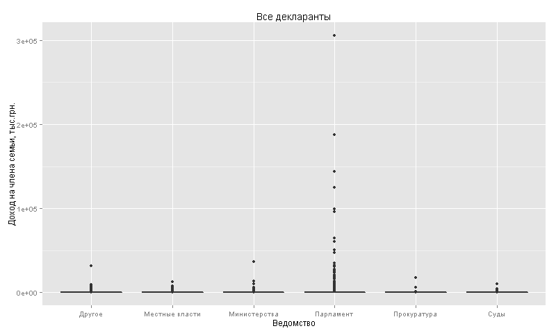
10%- , 10% - -: 10% — 305,8 .. ( 12 .), 90%- 382 ..
quantile(decl_df$income_per_member_ths, probs=seq(0,1,0.1))
:
qplot(data=decl_df, x=office_g, y = income_per_member_ths,
      geom="boxplot",
      xlab="",
      ylab="   , ..",
      main=" ")
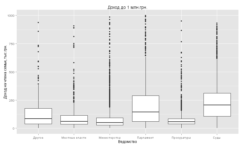
. 50 .. . 1 .. ( 97%):
qplot(data=decl_df[decl_df$income_per_member_ths<1000,],
      x=office_g, y = income_per_member_ths, geom="boxplot",
      xlab="",
      ylab="   , ..",
      main="  1 ..")
, (231 .) (209 .). 75-100 .. .
vs
, . .
# dataframe
decl_family<-decl_df[decl_df$number_of_family_members_incl_decl>1,]
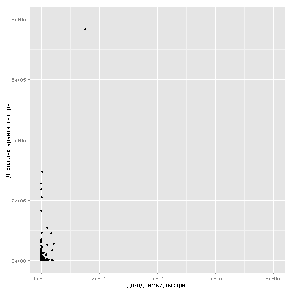
qplot(data=decl_family, y=income.own/1000, x=income.family/1000,
xlim=c(0,800000), ylim=c(0,800000),
xlab=" , ..", ylab=" , ..")
- . , ( 1 .. , — 94%):
nrow(decl_family[decl_family$income.own<1000000 & decl_family$income.family<1000000,])/nrow(decl_family)

qplot(data=decl_family, y=income.own/1000, x=income.family/1000,
      xlim=c(0,1000), ylim=c(0,1000),
      xlab=" , ..", ylab=" , ..",
      main="  1 ..")
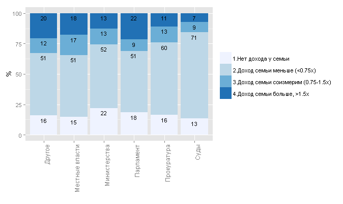
, ( ), , 77% — , 30% ( International Labour Organization)
(. ). , . — (, - ).
# -  4 :
#1.
#2.   75%
#3.      (  75%  150%  )
#4.      1,5

decl_family$family.own.income.ratio<-""

for (i in 1:nrow(decl_family))
{
  if (decl_family$income.family[i]==0)
  {decl_family$family.own.income.ratio[i]<-"1.   "}

  else
  {
    if (decl_family$income.family[i]<=0.75*decl_family$income.own[i])
    {decl_family$family.own.income.ratio[i]<-"2.   (<0.75x)"}

    else
    {
      if (decl_family$income.family[i]<=1.5*decl_family$income.own[i])
      {
        decl_family$family.own.income.ratio[i]<-"3.   (0.75-1.5)"
      }
      if (decl_family$income.family[i]>1.5*decl_family$income.own[i])
      {
        decl_family$family.own.income.ratio[i]<-"4.  , >1.5x"
      }
    }
  }
}

decl_family$family.own.income.ratio<-as.factor(decl_family$family.own.income.ratio)

#   %
y<-as.data.frame(100*prop.table(table(decl_family$family.own.income.ratio,decl_family$office_g), margin=2))

#
ggplot(y, aes(x = Var2, y = Freq, fill = Var1)) +
  geom_bar(stat="identity")+
  ylab("%") +
  xlab("")+
  theme(text = element_text(size=14), legend.title=element_blank(),axis.text.x = element_text(angle=90, size=12,vjust=1,hjust=1))+
  geom_text(aes(label = round(Freq,0),ymax=100),size=4,vjust=1.5,position="stack")+
  scale_fill_brewer()
?
— . , , .
— , 40% ( ).
, .
— , . , , . — .
, , — — . .
? . 1 .
, . 294 .
#   (  )
decl_df$income.own.and.family<-decl_df$income.own+decl_df$income.family

#      (.45-53 )
decl_df$banks<-decl_df$banks45+decl_df$banks47+decl_df$banks49+
              decl_df$banks51+decl_df$banks52+decl_df$banks53

#
decl_df$banks.income.ratio<-decl_df$banks/(decl_df$income.own.and.family+1)

#
#     ,
# 5    ,

decl_df$susp1<-0

for (i in 1:nrow(decl_df))
{
  if (decl_df$banks[i]>5*decl_df$income.own.and.family[i])
  {decl_df$susp1[i]<-1}
}
- . , , — , -, , -, , .
. 50 .
decl_df$susp2<-0

for (i in 1:nrow(decl_df))
{
  if (decl_df$income.own.and.family[i]==0)
  {decl_df$susp2[i]<-1}
}
- ,
, , , .
478 . 25% , 2 — 49 .
, , , .. — , - / , , .
#
decl_df$estate.own<-decl_df$estate24+decl_df$estate25+
                    decl_df$estate26+decl_df$estate27+decl_df$estate28
#
decl_df$estate.family<-decl_df$estate30+decl_df$estate31+
                    decl_df$estate32+decl_df$estate33+decl_df$estate34

#    25%
x<-quantile(decl_df[decl_df$number_of_family_members>0,]$income.family, probs=seq(0,1,0.25))[2]


#
y<-mean(decl_df[decl_df$number_of_family_members>0,]$estate.family)

#
#

decl_df$susp3<-0

for (i in 1:nrow(decl_df))
{
  if (decl_df$estate.family[i]>y & decl_df$estate.family[i]>decl_df$estate.own[i])
  {
    #        ,
    if (decl_df$income.family[i]<x)
    {decl_df$susp3[i]<-2}
    else
    {decl_df$susp3[i]<-1}
  }

}
- - ( )
128 , - ( ). 44 — .
# -  (  )
decl_df$income.from.abroad<-decl_df$income.own.21+as.double(decl_df$income.family.22)

decl_df$susp4<-0

for (i in 1:nrow(decl_df))
{
#  -  ,     —
if (decl_df$income.from.abroad[i]>
decl_df$income.own.and.family[i]-decl_df$income.from.abroad[i])
  {decl_df$susp4[i]<-1}
}
, . 31 .
#  (  )
decl_df$vehicles<-decl_df$vehicle35+decl_df$vehicle36+
                  decl_df$vehicle40+decl_df$vehicle41

decl_df$susp5<-0

for (i in 1:nrow(decl_df))
{
 if (decl_df$vehicles[i]>2 &  decl_df$estate.own[i]==0 & decl_df$estate.family[i]==0)
 {decl_df$susp5[i]<-1}
}
- , . - Luxury vehicle.
: Acura, Alfa Romeo Giulia, Audi A4, Audi A6, Audi A7, Audi A8, Bentley, BMW 3, BMW 5, BMW 7, Cadillac, Ferrari, Hummer, Infinity, Jaguar, Lamborghini, Land Rover, Lexus, Maserati, Mercedes-Benz C, Mercedes-Benz E, Mercedes-Benz GL, Mercedes-Benz S, Porsche, Rolls-Royce, Saab 9-3, Saab 9-5, Volkswagen Phaeton, Volvo S60, Volvo S80.
, , , ( , ). 653 .
#
luxury_cars<-c('Acura',	'Lexus',	'Cadillac',	'Alfa Romeo Giulia',	'Jaguar',	'Volvo S60',	'Infinity',	'Saab 9-3',	'BMW 3',	'Audi A4',	'Mercedes-Benz C',	'Volvo S80',	'Audi A6',	'Audi A7',	'Mercedes-Benz E',	'Saab 9-5',	'Maserati',	'BMW 5',	'BMW 7',	'Audi A8',	'Mercedes-Benz S',	'Porsche',	'Volkswagen Phaeton',	'Rolls-Royce',	'Bentley',	'Ferrari',	'Lamborghini',	'Mercedes-Benz GL',	'Hummer',	'Land Rover')

for (j in (1:nrow(decl_df)))
{
  decl_df$susp5.1[j]<-0
  for (i in (1:length(luxury_cars)))
  {
    #
    if (grepl(luxury_cars[i], decl_df$vehicle_names[j],
                  ignore.case=TRUE)==TRUE)
        {
            # -
            decl_df$susp5.1[j]<-decl_df$susp5.1[j]+
            length(gregexpr(luxury_cars[i], decl_df$vehicle_names[j],ignore.case=TRUE)[[1]])
        }
  }
}

decl_df$susp5.2<-0

#    -
for (i in (1:nrow(decl_df))) {if (decl_df$susp5.1[i]>0) decl_df$susp5.2[i]<-1}

#    -
for (i in (1:nrow(decl_df))) {if (decl_df$vehicles[i]==1) decl_df$susp5.2[i]<-0}
- .
, . 419 .
#    0
decl_df$familyPE.own.income.ratio<-0

# ,     ,
#
decl_df[decl_df$income.own.and.family>0,]$familyPE.own.income.ratio<-
decl_df[decl_df$income.own.and.family>0,]$income.family.17/decl_df[decl_df$income.own.and.family>0,]$income.own.and.family

#           .   ,
x<-mean(decl_df[decl_df$income.family.17>0,]$familyPE.own.income.ratio)

decl_df$susp6<-0

#    —

for (i in 1:nrow(decl_df))
{
  if (decl_df$familyPE.own.income.ratio[i]>x)
  {decl_df$susp6[i]<-1}
}
- ( garnahata)
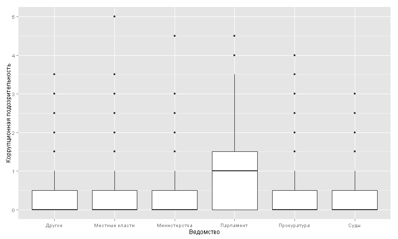
«» — .
— ( 80 ) 1 .
, ( ) , . , ( 2 ), 0,5 .
Excel,
, .
decl_df$suspicious<-decl_df$susp1+decl_df$susp2+
                    decl_df$susp3+decl_df$susp4+decl_df$susp5+decl_df$susp5.2+
                    decl_df$susp6+decl_df$hata_own+decl_df$hata_family*0.5
10 346 3971, — 0,5 1461 . — 5 ( 9,5).
:
Source: https://habr.com/ru/post/271773/
All Articles