Writing FEM calculator in less than 180 lines of code
Nowadays, FEM is probably the most common method for solving a wide range of applied engineering problems. Historically, it appeared from mechanics, but was subsequently applied to all kinds of non-mechanical tasks.
Today there is a wide variety of software packages, such as ANSYS , Abaqus , Patran , Cosmos , etc. These software packages allow you to solve problems of structural mechanics, fluid mechanics, thermodynamics, electrodynamics, and many others. The implementation of the method itself, as a rule, is considered rather complicated and voluminous.
Here I want to show that at present, using modern tools, writing the simplest FEM calculator from scratch for a two-dimensional problem of a plane-stressed state is not something very complicated and cumbersome. I chose this type of problem because it was the first successful example of the application of the finite element method. And of course it is the easiest to implement. I am going to use a linear, three-node element, since it is the only flat element in which case no numerical integration is required, as will be shown below. For elements of a higher order, with the exception of the integration operation (which is not quite trivial, but its implementation is quite interesting), the idea is absolutely the same.
')
Picture to attract attention:
Historically, the first practical application of FEM was in the field of mechanics, which significantly affected the terminology and the first interpretations of the method. In the simplest case, the essence of the method can be described as follows: the continuum is replaced by an equivalent hinge system, and the solution of statically indefinable systems is a well-known and studied problem of mechanics. This simplified, engineering interpretation has contributed to the widespread dissemination of the method, but strictly speaking, this understanding of the method is incorrect. The exact mathematical substantiation of the method was given much later than the first successful applications of the method, but this made it possible to expand the field of application for a larger range of tasks, not only from the field of mechanics.
I am not going to describe the method in detail, there is a lot of literature about it, instead I will focus on the implementation of the method. Minimum knowledge of mechanics, or the same strength of materials, will be required. I will also be happy if reviews from people who are not related to mechanics, if at least the idea was clear. The implementation of the method will be in C ++, however, I will not use any strongly specific features of this language and I hope that the code will be understood by people who do not know this language.
Since this is just an example of the implementation of the method, so as not to complicate and leave everything in the most simple form to understand, I will prefer brevity at the expense of many programming principles. This is not an example of writing good, maintained and reliable code; it is an example of the implementation of the FEM. So there will be many simplifications to concentrate on the main goal.
Before proceeding to the method itself, let's find out in what form we will represent the input data. The object under consideration should be divided into a large number of small elements, in our case - triangles. Thus, we replace the continuous medium with a set of nodes and finite elements that form a grid. The figure below shows an example of a grid with numbered nodes and elements.
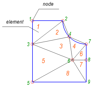
In the figure we see nine nodes and eight elements. To describe the grid, you need two lists:
In the list of elements, each element is defined by the set of indexes of the nodes that form the element. In our case, we only have triangular elements, so we will use only three indexes for each element.
As an example, for the grid shown above, we will have the following lists:
List of nodes:
List of items:
It is worth noting that there are several ways to specify the same element. Node indices can be listed clockwise or counterclockwise. The counterclockwise enumeration is usually used, so we will assume that all elements are defined in this way.
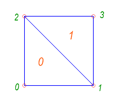
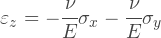
Let's create some input file with a complete description of the task. To avoid confusion and not complicate, it is better to use indexing, which starts from zero, and not from one, because in C / C ++ arrays are indexed from zero. For the first test input file, we will create the simplest possible grid:
Let the first line be a description of the properties of the material. For example, for steel, the Poisson's ratio is ν = 0.3 and the Young's modulus is E = 2000 MPa:
Then follows a line with the number of nodes and then the list of nodes:
Then follows a line with the number of elements, then a list of elements:
Now, we need to specify constraints, or as they say, conditions on the border of the first kind. As such boundary conditions, we will fix the displacements of the nodes. It is possible to fix movements along the axes independently of each other, i.e. we can prohibit movement along the x axis or along the y axis or both at once. In general, you can specify some initial displacement, however, we restrict ourselves to only zero initial displacement. Thus, we will have a list of nodes with a given type of movement restrictions. The type of restriction will be indicated by the number:
The first line defines the number of restrictions:
Then, we have to set the load. We will work only with the nodal forces. Strictly speaking, the nodal forces should not be viewed as forces in the general sense of the word; I will talk about this later, but for now let's think of them simply as forces acting on a node. We need a list with indexes of nodes and corresponding force vectors. The first line defines the number of applied forces:
It is easy to see that the task in question is a square-shaped body, the bottom of which is fixed, and tensile forces act on the upper edge.

Full input file:
Before I start writing the code, I would like to talk about the mathematical library - Eigen . It is a mature, reliable and efficient library that has a very clean and expressive API. There are many compile-time optimizations in it, the library is able to perform explicit vectoring and supports SSE 2/3/4, ARM and NEON instructions. As for me, this library is remarkable at least in that it allows you to implement complex mathematical calculations in a brief and expressive way.
I would like to make a brief description of the part of the Eigen API, which we will use below. Readers who are familiar with this library may skip this section.
There are two types of matrices: dense and sparse. We will use both types. In the case of a dense matrix, all elements are in memory, in the order of the indices, both column-major (default) and raw-major placement are supported. This type of matrix is good for relatively small matrices or matrices with a small number of zero elements. Sparse matrices are good for storing large matrices with a small number of non-zero elements. We will use a sparse matrix for the global stiffness matrix.
To use dense matrices, we will need to include the <Eigen / Dense> header. There are two main types of dense matrices: with fixed and with dynamic size. A fixed-size matrix is a matrix whose size is known at compile time. In the case of a matrix of dynamic size, its size can be specified at the stage of code execution, moreover, the size of the dynamic matrix can even be changed on the fly. Of course, you need to give preference to matrices with a fixed size wherever possible. Memory for dynamic matrices is allocated on the heap, and the unknown size of the matrix limits the optimizations that the compiler can do. Fixed matrices can be allocated on the stack, the compiler can expand loops and much more. It should be noted that a mixed type is also possible, when the number of rows in the matrix is fixed, but the number of columns is dynamic, or vice versa.
Fixed-size matrices can be defined as follows:
Where m is the float matrix c of fixed sizes of 3 × 3. You can also use the following predefined types:
There are a few more predefined types, these are basic. The number indicates the dimension of the square matrix and the letter indicates the type of the matrix element: i is an integer, f is a single-precision floating-point number, d is a double-precision floating-point number.
For vectors there is no separate type, vectors are the same matrices. The column vector (sometimes in the literature there are row vectors, you have to specify), you can declare as follows:
Or you can use one of the predefined types (the notation is the same as for matrices):
For quick reference, I wrote the following example:
Conclusion:
For more information, it is better to consult the documentation .
Sparse matrix is a bit more complex type of matrix. The basic idea is not to keep the entire matrix in memory as it is, but to store only non-zero elements. Quite often in practical problems there are large matrices with a small number of nonzero elements. When assembling the global stiffness matrix in the FEM model, the number of nonzero elements can be less than 0.1% of the total number of elements.
For modern FEM packages, it’s not a problem to solve a problem with hundreds of thousands of nodes, and on a completely ordinary modern PC. If we try to allocate space for storing the global stiffness matrix, we will encounter the following problem:

The size of the memory required to store the matrix is huge! A thin matrix would require 10,000 times less memory.
Sparse matrices use memory more efficiently because they store only nonzero elements. Sparse matrices can be represented in two ways: compressed and uncompressed. In uncompressed form, it is easy to add or remove an element from the matrix, but this type of representation is not optimal in terms of memory usage. Eigen, when working with a sparse matrix, uses a kind of compressed representation, somewhat more optimized for the dynamic addition / removal of elements. Eigen is also able to convert such a matrix into a compressed form, moreover, it does this transparently, it is not necessary to do this explicitly. Most algorithms require a compressed matrix view, and the use of any of these algorithms automatically converts the matrix into a compressed form. Conversely, adding / removing an item automatically converts the matrix into an optimized view.
How can we define a matrix? A good way to do this is to use the so-called Triplets . This is a data structure, and this is a template class, which is a single element of the matrix in combination with indices determining its position in the matrix. We can specify a sparse matrix directly from the triplets vector.
For example, we have the following sparse matrix:
The first thing we need to do is include the appropriate Eigen library header: <Eigen / Sparse> . Then, we declare an empty sparse matrix of dimension 5x5. Next, we define the triplets vector and fill it with values. The triplet 's constructor takes the following arguments: i-index, j-index, value.
The output will be as follows:
To store the data we are going to read from the input file, as well as intermediate data, we must declare our structures. The simplest data structure describing the final element is shown below. It consists of an array of three elements that store the indexes of the nodes forming the final element, as well as the matrix B. This matrix is called the gradient matrix and we will return to it later. The CalculateStiffnessMatrix method will also be described below.
Another simple structure that we need is a structure for describing attachments. This is a simple structure consisting of an enumerated type, which determines the type of restriction, and the index of the node on which the restriction is imposed.
To keep things simple, let's define some global variables. Creating any global objects is always a bad idea, but for this example it’s perfectly acceptable. We will need the following global variables:
In the code, we define them as follows:
Before reading something like something, we need to know where to read and where to write the output. At the beginning of the main function, check the number of input arguments, note that the first argument is always the path to the executable file. Thus, we should have three arguments, even if the second is the path to the input file, and the third is the path to the file with the output. To work with I / O, for a particular case the most convenient way is to use file streams from the standard library.
The first thing we do is create streams for I / O:
In the first line of the input file are the properties of the material, read them:
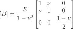
This is enough to build an elastic matrix of an isotropic material for a plane-stressed state, which is defined as follows:

Where did these expressions come from? They are easily obtained from Hooke’s law in a general form; indeed, we can find an expression for the matrix D from the following relations:
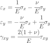
It should be noted that the plane-stressed state means that σ Z is zero, but not ε Z. A plane-stressed model is well suited for solving a number of engineering problems, where flat structures are considered and all forces act in the plane. At a time when calculations of volumetric problems were too expensive, many tasks could be reduced to flat ones, while sacrificing accuracy.
In a plane-stressed state, nothing prevents the body from deforming in the direction normal to its plane; therefore, the deformation ε Z is generally not equal to zero. It does not appear in the equations above, but can be easily obtained from the following relationship, given that the stress σ Z is zero:
We have all the initial data to set the elastic matrix, let's do it:
Next, we read the list with the coordinates of the nodes. First we read the number of nodes, then we set the size of the dynamic vectors x and y. Next, we just read the coordinates of the nodes in the loop, line by line.
Then, we read the list of items. All the same, read the number of elements, and then the indexes of the nodes for each element:
Next, read the list of posts. All the same:
You may have noticed static_cast , it is needed to convert an int type, to the previously declared enumerated type for assignments.
Finally, you need to read the list of loads. There is one feature associated with the load, because of which we will represent the actual load in the form of a vector of dimension of double the number of nodes. The reason why we do this will be explained later. The figure below illustrates this load vector:
Thus, for each node, we have two elements in the load vector that represent the x and y components of the force. Thus, the x-component of the effort in a certain node will be stored in the element with the id = 2 * node_id + 0 index, and the y-component of the force for this node will be stored in the element with the id = 2 * node_id + 1 index.
First, we set the size of the vector of applied efforts twice as large as the number of nodes, then zero the vector. We read the number of external forces and read their values line by line:
We consider a geometrically linear system with infinitesimal displacements. Moreover, we assume that the deformation occurs elastically, i.e. deformations are a linear function of stress (Hooke's law). , . , , :
: — ; δ — ; R — , . , , .
, :

: u i v i — u- v- i- .
:

: R xi R yi- the x-component and the y-component of the external force applied to the i-th node.
As we see, each element of the displacement vector and load vector is a two-dimensional vector. Instead, we can define these vectors as follows:
That is actually the same, but it simplifies the representation of these vectors in the code. This is an explanation of why we previously set the load vector in such a peculiar way.
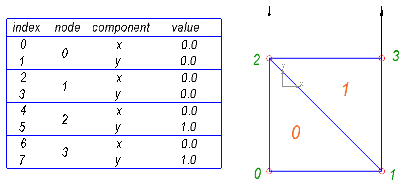
How to build a stiffness matrix? The essence of the global stiffness matrix is a superposition of the stiffness matrices of each element. If we consider one element separately from the others, then we can determine the same stiffness matrix, but only for this element. This matrix defines the relationship between node movements and nodal forces. For example, for a 3-node element:
Where: [k] — e- ; [δ] — - ; [F] — - ; i, j, m — .
, ? , - , . , , , — .
The sum of all the nodal forces at each node is equal to the sum of the external forces at that node, this follows from the equilibrium principle. Despite the fact that this statement may seem quite logical and fair, in fact, everything is a bit more complicated. Such a formulation is not accurate, because the nodal forces are not forces in the general sense of the word, and the fulfillment of the equilibrium conditions is not an obvious condition for them. Despite the fact that the statement is still true, it uses a mechanical principle, which limits the application of the method. There is a more rigorous, mathematical justification of the FEM from the standpoint of minimizing potential energy, which makes it possible to extend the method to a wider range of problems.
, , . , , , . , , , ( ), , .
, - . — . , , :
:

, triplets . , :
std::vector<Eigen::Triplet<float> > — triplets ; CalculateStiffnessMatrix — , triplets .
, triplets :
, () , .
. , :
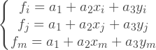
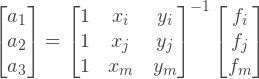
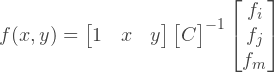
[N] (, ) . . , u v , , :
:


? , . -, , . :

f , :
:

, :
, :
, , :

, :
Knowing the displacement field, we can find the strain field on the relations of the theory of elasticity:
Now we can replace u and v , in the form of functions:

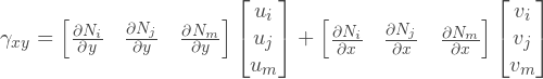
Or we can write the same in combined form:

The matrix on the right side, commonly referred to as a matrix in , the so-called gradient matrix.
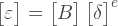
To find the matrix B , we must find all partial derivatives of the functions of the form:

In the case of a linear element, we see that the partial derivatives of the functions of the form are in fact constants, which will save us a lot of effort, as will be shown later. Multiplying the row vector with constants by the inverse matrix C we get:


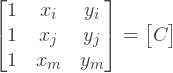
Now we can calculate the B matrix. To build the matrix C, we first define the coordinate vectors of the nodes:
Then, we can build a matrix C of three rows:
Then we compute the inverse matrix C and collect the matrix B:
, D:

, , :
, , . . , , . , . , , .
, , . , : d[δ] e
, . , , , . , , , .
, :
- :

Or:
, :
, :

, , :
, . , , , :
, , . , :

A — , t — . , :
, :
, . , : , 2 . , , , . , . , .
CalculateStiffnessMatrix :
, , Triplets . Triplet , . , , , — , — .
The resulting system of linear equations cannot be solved until we specify the fixings. Purely from a mechanical point of view, an unsecured system can make any large displacements, and under the action of external forces, it can even go into motion. Mathematically, this will lead to the fact that the resulting SLAE is not linearly independent, and therefore does not have a unique solution.
Moves of some nodes must be set to zero or to some predetermined value. In the simplest case, let's consider only the fixing of the nodes, without initial displacements. In fact, this means that we remove some equations from the system. But changing the number of equations of the system on the fly is not a trivial task. Instead, you can use the following trick.
Let's say we have the following system of equations:
To fix a node, the corresponding matrix element must be set to 1, and all elements in the row and column containing this element must be set to zero. There should also be no external forces acting on the fixed node in the direction in which the restriction is valid. An equation with this node will explicitly give a zero offset for this node, and the zeros in the corresponding column will exclude this offset from other equations. Let's say we want to fix the zero node in the direction of the x axis, and fix the first node in the direction of the y axis:

To perform this operation, we first define the indices of the equations that we are going to exclude from the SLAE. To do this, we loop through the list of assignments and collect the vector of indices. Then, going through all the nonzero elements of the stiffness matrix, we call the function SetConstraints . The following is the ApplyConstraints function :
The SetConstraints function checks whether an element of the stiffness matrix is part of the excluded equation, and if so, it sets it equal to zero or one, depending on whether the element is on the diagonal or not:
Further, we simply call ApplyConstraints and pass as its arguments a global stiffness matrix and a vector of constraints:
The Eigen library has various sparse linear equations solvers available, we will use SimplicialLDLT , which is a fast direct solver. For demonstration purposes, we will derive the initial stiffness matrix and load vector, and then output the result of the solution, the displacement vector.
Of course, the matrix output makes sense only for our test example, which contains only two elements.
As we have seen before, we can move from displacements to deformations and further to stresses:
However, we obtain a stress vector, which in theory of elasticity is generally a second-rank symmetric tensor:

As you know, the tensor elements directly depend on the coordinate system, however the physical state itself is of course independent. Therefore, for analysis, it is better to proceed as an invariant value, best of all, to a scalar one. Such an invariant is the von Mises stresses :
, - , . , , , .
, :
. , :
, , . , . x-, 0.0003, 0.3 y-, . , .
cloc :
, — 171 .
, python, . , PIL , . Abaqus , , .
:
, Abaqus . Abaqus ' . .
Here we see a strip with a hole, the bottom of which is fixed, and a tensile force is applied to the upper edge:
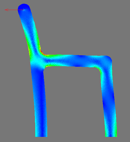
Abstract structural element, just for beauty. The bottom of the structure is fixed, and a concentrated force is applied on the upper protruding part, which I have already drawn on top of the picture:
Another example with a strip with a hole, this time only a quarter of the structure is considered due to symmetry. The left border is fixed along the x axis, the lower one along the y axis. The maximum voltage received: 3.05152. This value, despite the coarseness of the grid (and perhaps because of it), is quite close to the theoretical value - 3.
The same problem, but solved in Abaqus. As you can see, the maximum voltage is 3.052, which fully coincides with our result. Such an exact coincidence, in principle, is not surprising, since in practice, it is difficult for a triangular element to do something in some way, so that the result is different. For elements of a higher order, unfortunately, such a 100% coincidence did not work out for me, which can be explained by different implementation of numerical integration.
All source code, including examples, is available on github .
Honestly, behind the scenes there are quite a lot. But the article turned out to be inflated, and so I think this can be stopped.
Not included (but wanted):
, , , MATLAB , ++. , , , .. . , , .
PS , , .
Today there is a wide variety of software packages, such as ANSYS , Abaqus , Patran , Cosmos , etc. These software packages allow you to solve problems of structural mechanics, fluid mechanics, thermodynamics, electrodynamics, and many others. The implementation of the method itself, as a rule, is considered rather complicated and voluminous.
Here I want to show that at present, using modern tools, writing the simplest FEM calculator from scratch for a two-dimensional problem of a plane-stressed state is not something very complicated and cumbersome. I chose this type of problem because it was the first successful example of the application of the finite element method. And of course it is the easiest to implement. I am going to use a linear, three-node element, since it is the only flat element in which case no numerical integration is required, as will be shown below. For elements of a higher order, with the exception of the integration operation (which is not quite trivial, but its implementation is quite interesting), the idea is absolutely the same.
')
Picture to attract attention:
Historically, the first practical application of FEM was in the field of mechanics, which significantly affected the terminology and the first interpretations of the method. In the simplest case, the essence of the method can be described as follows: the continuum is replaced by an equivalent hinge system, and the solution of statically indefinable systems is a well-known and studied problem of mechanics. This simplified, engineering interpretation has contributed to the widespread dissemination of the method, but strictly speaking, this understanding of the method is incorrect. The exact mathematical substantiation of the method was given much later than the first successful applications of the method, but this made it possible to expand the field of application for a larger range of tasks, not only from the field of mechanics.
I am not going to describe the method in detail, there is a lot of literature about it, instead I will focus on the implementation of the method. Minimum knowledge of mechanics, or the same strength of materials, will be required. I will also be happy if reviews from people who are not related to mechanics, if at least the idea was clear. The implementation of the method will be in C ++, however, I will not use any strongly specific features of this language and I hope that the code will be understood by people who do not know this language.
Since this is just an example of the implementation of the method, so as not to complicate and leave everything in the most simple form to understand, I will prefer brevity at the expense of many programming principles. This is not an example of writing good, maintained and reliable code; it is an example of the implementation of the FEM. So there will be many simplifications to concentrate on the main goal.
Input data
Before proceeding to the method itself, let's find out in what form we will represent the input data. The object under consideration should be divided into a large number of small elements, in our case - triangles. Thus, we replace the continuous medium with a set of nodes and finite elements that form a grid. The figure below shows an example of a grid with numbered nodes and elements.
In the figure we see nine nodes and eight elements. To describe the grid, you need two lists:
- A list of nodes that defines the coordinates of each node.
- List of items.
In the list of elements, each element is defined by the set of indexes of the nodes that form the element. In our case, we only have triangular elements, so we will use only three indexes for each element.
As an example, for the grid shown above, we will have the following lists:
List of nodes:
0.000000 31.500000 15.516667 31.500000 0.000000 19.489759 18.804134 23.248226 0.000000 0.000000 20.479981 11.365822 27.516667 19.500000 27.516667 11.365822 27.516667 0.000000 List of items:
1 3 2 2 3 4 4 6 7 4 3 6 7 6 8 3 5 6 6 5 9 6 9 8 It is worth noting that there are several ways to specify the same element. Node indices can be listed clockwise or counterclockwise. The counterclockwise enumeration is usually used, so we will assume that all elements are defined in this way.
Let's create some input file with a complete description of the task. To avoid confusion and not complicate, it is better to use indexing, which starts from zero, and not from one, because in C / C ++ arrays are indexed from zero. For the first test input file, we will create the simplest possible grid:
Let the first line be a description of the properties of the material. For example, for steel, the Poisson's ratio is ν = 0.3 and the Young's modulus is E = 2000 MPa:
0.3 2000 Then follows a line with the number of nodes and then the list of nodes:
4 0.0 0.0 1.0 0.0 0.0 1.0 1.0 1.0 Then follows a line with the number of elements, then a list of elements:
2 0 1 2 1 3 2 Now, we need to specify constraints, or as they say, conditions on the border of the first kind. As such boundary conditions, we will fix the displacements of the nodes. It is possible to fix movements along the axes independently of each other, i.e. we can prohibit movement along the x axis or along the y axis or both at once. In general, you can specify some initial displacement, however, we restrict ourselves to only zero initial displacement. Thus, we will have a list of nodes with a given type of movement restrictions. The type of restriction will be indicated by the number:
- 1 - movement in the direction of the x axis is prohibited
- 2 - movement in the direction of the y axis is prohibited
- 3 - moving in both, x and y directions is prohibited
The first line defines the number of restrictions:
2 0 3 1 2 Then, we have to set the load. We will work only with the nodal forces. Strictly speaking, the nodal forces should not be viewed as forces in the general sense of the word; I will talk about this later, but for now let's think of them simply as forces acting on a node. We need a list with indexes of nodes and corresponding force vectors. The first line defines the number of applied forces:
2 2 0.0 1.0 3 0.0 1.0 It is easy to see that the task in question is a square-shaped body, the bottom of which is fixed, and tensile forces act on the upper edge.
Full input file:
0.3 2000 4 0.0 0.0 1.0 0.0 0.0 1.0 1.0 1.0 2 0 1 2 1 3 2 2 0 3 1 2 2 2 0.0 1.0 3 0.0 1.0 Eigen - Mathematical Library
Before I start writing the code, I would like to talk about the mathematical library - Eigen . It is a mature, reliable and efficient library that has a very clean and expressive API. There are many compile-time optimizations in it, the library is able to perform explicit vectoring and supports SSE 2/3/4, ARM and NEON instructions. As for me, this library is remarkable at least in that it allows you to implement complex mathematical calculations in a brief and expressive way.
I would like to make a brief description of the part of the Eigen API, which we will use below. Readers who are familiar with this library may skip this section.
There are two types of matrices: dense and sparse. We will use both types. In the case of a dense matrix, all elements are in memory, in the order of the indices, both column-major (default) and raw-major placement are supported. This type of matrix is good for relatively small matrices or matrices with a small number of zero elements. Sparse matrices are good for storing large matrices with a small number of non-zero elements. We will use a sparse matrix for the global stiffness matrix.
Dense matrices
To use dense matrices, we will need to include the <Eigen / Dense> header. There are two main types of dense matrices: with fixed and with dynamic size. A fixed-size matrix is a matrix whose size is known at compile time. In the case of a matrix of dynamic size, its size can be specified at the stage of code execution, moreover, the size of the dynamic matrix can even be changed on the fly. Of course, you need to give preference to matrices with a fixed size wherever possible. Memory for dynamic matrices is allocated on the heap, and the unknown size of the matrix limits the optimizations that the compiler can do. Fixed matrices can be allocated on the stack, the compiler can expand loops and much more. It should be noted that a mixed type is also possible, when the number of rows in the matrix is fixed, but the number of columns is dynamic, or vice versa.
Fixed-size matrices can be defined as follows:
Eigen::Matrix<float, 3, 3> m; Where m is the float matrix c of fixed sizes of 3 × 3. You can also use the following predefined types:
Eigen::Matrix2i Eigen::Matrix3i Eigen::Matrix4i Eigen::Matrix2f Eigen::Matrix3f Eigen::Matrix4f Eigen::Matrix2d Eigen::Matrix3d Eigen::Matrix4d There are a few more predefined types, these are basic. The number indicates the dimension of the square matrix and the letter indicates the type of the matrix element: i is an integer, f is a single-precision floating-point number, d is a double-precision floating-point number.
For vectors there is no separate type, vectors are the same matrices. The column vector (sometimes in the literature there are row vectors, you have to specify), you can declare as follows:
Eigen::Matrix<float, 3, 1> v; Or you can use one of the predefined types (the notation is the same as for matrices):
Eigen::Vector2i Eigen::Vector3i Eigen::Vector4i Eigen::Vector2f Eigen::Vector3f Eigen::Vector4f Eigen::Vector2d Eigen::Vector3d Eigen::Vector4d For quick reference, I wrote the following example:
#include <iostream> int main() { //Fixed size 3x3 matrix of floats Eigen::Matrix3f A; A << 1, 0, 1, 2, 5, 0, 1, 1, 2; std::cout << "Matrix A:" << std::endl << A << std::endl; //Access to matrix element [1, 1]: std::cout << "A[1, 1]:" << std::endl << A(1, 1) << std::endl; //Fixed size 3 vector of floats Eigen::Vector3f B; B << 1, 0, 1; std::cout << "Vector B:" << std::endl << B << std::endl; //Access to vector element [1]: std::cout << "B[1]:" << std::endl << B(1) << std::endl; //Multiplication of vector and matrix Eigen::Vector3f C = A * B; std::cout << "C = A * B:" << std::endl << C << std::endl; //Dynamic size matrix of floats Eigen::MatrixXf D; D.resize(3, 3); //Let matrix D be an identity matrix: D.setIdentity(); std::cout << "Matrix D:" << std::endl << D << std::endl; //Multiplication of matrix and matrix Eigen::MatrixXf E = A * D; std::cout << "E = A * D:" << std::endl << E << std::endl; return 0; } Conclusion:
Matrix A: 1 0 1 2 5 0 1 1 2 A[1, 1]: 5 Vector B: 1 0 1 B[1]: 0 C = A * B: 2 2 3 Matrix D: 1 0 0 0 1 0 0 0 1 E = A * D: 1 0 1 2 5 0 1 1 2 For more information, it is better to consult the documentation .
Sparse matrix
Sparse matrix is a bit more complex type of matrix. The basic idea is not to keep the entire matrix in memory as it is, but to store only non-zero elements. Quite often in practical problems there are large matrices with a small number of nonzero elements. When assembling the global stiffness matrix in the FEM model, the number of nonzero elements can be less than 0.1% of the total number of elements.
For modern FEM packages, it’s not a problem to solve a problem with hundreds of thousands of nodes, and on a completely ordinary modern PC. If we try to allocate space for storing the global stiffness matrix, we will encounter the following problem:
The size of the memory required to store the matrix is huge! A thin matrix would require 10,000 times less memory.
Sparse matrices use memory more efficiently because they store only nonzero elements. Sparse matrices can be represented in two ways: compressed and uncompressed. In uncompressed form, it is easy to add or remove an element from the matrix, but this type of representation is not optimal in terms of memory usage. Eigen, when working with a sparse matrix, uses a kind of compressed representation, somewhat more optimized for the dynamic addition / removal of elements. Eigen is also able to convert such a matrix into a compressed form, moreover, it does this transparently, it is not necessary to do this explicitly. Most algorithms require a compressed matrix view, and the use of any of these algorithms automatically converts the matrix into a compressed form. Conversely, adding / removing an item automatically converts the matrix into an optimized view.
How can we define a matrix? A good way to do this is to use the so-called Triplets . This is a data structure, and this is a template class, which is a single element of the matrix in combination with indices determining its position in the matrix. We can specify a sparse matrix directly from the triplets vector.
For example, we have the following sparse matrix:
0 3 0 0 0 22 0 0 0 0 0 5 0 1 0 0 0 0 0 0 0 0 14 0 8 The first thing we need to do is include the appropriate Eigen library header: <Eigen / Sparse> . Then, we declare an empty sparse matrix of dimension 5x5. Next, we define the triplets vector and fill it with values. The triplet 's constructor takes the following arguments: i-index, j-index, value.
#include <Eigen/Sparse> #include <iostream> int main() { Eigen::SparseMatrix<int> A(5, 5); std::vector< Eigen::Triplet<int> > triplets; triplets.push_back(Eigen::Triplet<int>(0, 1, 3)); triplets.push_back(Eigen::Triplet<int>(1, 0, 22)); triplets.push_back(Eigen::Triplet<int>(2, 1, 5)); triplets.push_back(Eigen::Triplet<int>(2, 3, 1)); triplets.push_back(Eigen::Triplet<int>(4, 2, 14)); triplets.push_back(Eigen::Triplet<int>(4, 4, 8)); A.setFromTriplets(triplets.begin(), triplets.end()); A.insert(0, 0); std::cout << A; A.makeCompressed(); std::cout << std::endl << A; } The output will be as follows:
Nonzero entries: (0,0) (22,1) (_,_) (3,0) (5,2) (_,_) (_,_) (14,4) (_,_) (_,_) (1,2) (_,_) (_,_) (8,4) (_,_) (_,_) Outer pointers: 0 3 7 10 13 $ Inner non zeros: 2 2 1 1 1 $ 0 3 0 0 0 22 0 0 0 0 0 5 0 1 0 0 0 0 0 0 0 0 14 0 8 Nonzero entries: (0,0) (22,1) (3,0) (5,2) (14,4) (1,2) (8,4) Outer pointers: 0 2 4 5 6 $ 0 3 0 0 0 22 0 0 0 0 0 5 0 1 0 0 0 0 0 0 0 0 14 0 8 Data structures
To store the data we are going to read from the input file, as well as intermediate data, we must declare our structures. The simplest data structure describing the final element is shown below. It consists of an array of three elements that store the indexes of the nodes forming the final element, as well as the matrix B. This matrix is called the gradient matrix and we will return to it later. The CalculateStiffnessMatrix method will also be described below.
struct Element { void CalculateStiffnessMatrix(const Eigen::Matrix3f& D, std::vector<Eigen::Triplet<float> >& triplets); Eigen::Matrix<float, 3, 6> B; int nodesIds[3]; }; Another simple structure that we need is a structure for describing attachments. This is a simple structure consisting of an enumerated type, which determines the type of restriction, and the index of the node on which the restriction is imposed.
struct Constraint { enum Type { UX = 1 << 0, UY = 1 << 1, UXY = UX | UY }; int node; Type type; }; To keep things simple, let's define some global variables. Creating any global objects is always a bad idea, but for this example it’s perfectly acceptable. We will need the following global variables:
- Number of nodes
- Vector with x-coordinate of nodes
- Vector with y-coordinate of nodes
- Elements Vector
- Pinning vector
- Load vector
In the code, we define them as follows:
int nodesCount; int noadsCount; Eigen::VectorXf nodesX; Eigen::VectorXf nodesY; Eigen::VectorXf loads; std::vector< Element > elements; std::vector< Constraint > constraints; Read input file
Before reading something like something, we need to know where to read and where to write the output. At the beginning of the main function, check the number of input arguments, note that the first argument is always the path to the executable file. Thus, we should have three arguments, even if the second is the path to the input file, and the third is the path to the file with the output. To work with I / O, for a particular case the most convenient way is to use file streams from the standard library.
The first thing we do is create streams for I / O:
int main(int argc, char *argv[]) { if ( argc != 3 ) { std::cout << "usage: " << argv[0] << " <input file> <output file>\n"; return 1; } std::ifstream infile(argv[1]); std::ofstream outfile(argv[2]); In the first line of the input file are the properties of the material, read them:
float poissonRatio, youngModulus; infile >> poissonRatio >> youngModulus; This is enough to build an elastic matrix of an isotropic material for a plane-stressed state, which is defined as follows:
Where did these expressions come from? They are easily obtained from Hooke’s law in a general form; indeed, we can find an expression for the matrix D from the following relations:
It should be noted that the plane-stressed state means that σ Z is zero, but not ε Z. A plane-stressed model is well suited for solving a number of engineering problems, where flat structures are considered and all forces act in the plane. At a time when calculations of volumetric problems were too expensive, many tasks could be reduced to flat ones, while sacrificing accuracy.
In a plane-stressed state, nothing prevents the body from deforming in the direction normal to its plane; therefore, the deformation ε Z is generally not equal to zero. It does not appear in the equations above, but can be easily obtained from the following relationship, given that the stress σ Z is zero:
We have all the initial data to set the elastic matrix, let's do it:
Eigen::Matrix3f D; D << 1.0f, poissonRatio, 0.0f, poissonRatio, 1.0, 0.0f, 0.0f, 0.0f, (1.0f - poissonRatio) / 2.0f; D *= youngModulus / (1.0f - pow(poissonRatio, 2.0f)); Next, we read the list with the coordinates of the nodes. First we read the number of nodes, then we set the size of the dynamic vectors x and y. Next, we just read the coordinates of the nodes in the loop, line by line.
infile >> nodesCount; nodesX.resize(nodesCount); nodesY.resize(nodesCount); for (int i = 0; i < nodesCount; ++i) { infile >> nodesX[i] >> nodesY[i]; } Then, we read the list of items. All the same, read the number of elements, and then the indexes of the nodes for each element:
int elementCount; infile >> elementCount; for (int i = 0; i < elementCount; ++i) { Element element; infile >> element.nodesIds[0] >> element.nodesIds[1] >> element.nodesIds[2]; elements.push_back(element); } Next, read the list of posts. All the same:
int constraintCount; infile >> constraintCount; for (int i = 0; i < constraintCount; ++i) { Constraint constraint; int type; infile >> constraint.node >> type; constraint.type = static_cast<Constraint::Type>(type); constraints.push_back(constraint); } You may have noticed static_cast , it is needed to convert an int type, to the previously declared enumerated type for assignments.
Finally, you need to read the list of loads. There is one feature associated with the load, because of which we will represent the actual load in the form of a vector of dimension of double the number of nodes. The reason why we do this will be explained later. The figure below illustrates this load vector:
Thus, for each node, we have two elements in the load vector that represent the x and y components of the force. Thus, the x-component of the effort in a certain node will be stored in the element with the id = 2 * node_id + 0 index, and the y-component of the force for this node will be stored in the element with the id = 2 * node_id + 1 index.
First, we set the size of the vector of applied efforts twice as large as the number of nodes, then zero the vector. We read the number of external forces and read their values line by line:
int loadsCount; loads.resize(2 * nodesCount); loads.setZero(); infile >> loadsCount; for (int i = 0; i < loadsCount; ++i) { int node; float x, y; infile >> node >> x >> y; loads[2 * node + 0] = x; loads[2 * node + 1] = y; } Calculation of the global stiffness matrix
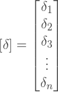
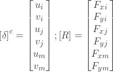
We consider a geometrically linear system with infinitesimal displacements. Moreover, we assume that the deformation occurs elastically, i.e. deformations are a linear function of stress (Hooke's law). , . , , :
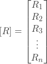
: — ; δ — ; R — , . , , .
, :
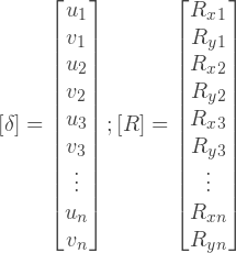
: u i v i — u- v- i- .
:
: R xi R yi- the x-component and the y-component of the external force applied to the i-th node.
As we see, each element of the displacement vector and load vector is a two-dimensional vector. Instead, we can define these vectors as follows:
That is actually the same, but it simplifies the representation of these vectors in the code. This is an explanation of why we previously set the load vector in such a peculiar way.
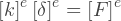
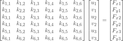
How to build a stiffness matrix? The essence of the global stiffness matrix is a superposition of the stiffness matrices of each element. If we consider one element separately from the others, then we can determine the same stiffness matrix, but only for this element. This matrix defines the relationship between node movements and nodal forces. For example, for a 3-node element:
Where: [k] — e- ; [δ] — - ; [F] — - ; i, j, m — .
, ? , - , . , , , — .
The sum of all the nodal forces at each node is equal to the sum of the external forces at that node, this follows from the equilibrium principle. Despite the fact that this statement may seem quite logical and fair, in fact, everything is a bit more complicated. Such a formulation is not accurate, because the nodal forces are not forces in the general sense of the word, and the fulfillment of the equilibrium conditions is not an obvious condition for them. Despite the fact that the statement is still true, it uses a mechanical principle, which limits the application of the method. There is a more rigorous, mathematical justification of the FEM from the standpoint of minimizing potential energy, which makes it possible to extend the method to a wider range of problems.
, , . , , , . , , , ( ), , .
, - . — . , , :
:
, triplets . , :
std::vector<Eigen::Triplet<float> > triplets; for (std::vector<Element>::iterator it = elements.begin(); it != elements.end(); ++it) { it->CalculateStiffnessMatrix(D, triplets); } std::vector<Eigen::Triplet<float> > — triplets ; CalculateStiffnessMatrix — , triplets .
, triplets :
Eigen::SparseMatrix<float> globalK(2 * nodesCount, 2 * nodesCount); globalK.setFromTriplets(triplets.begin(), triplets.end()); , () , .
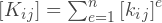
. , :
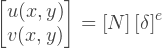
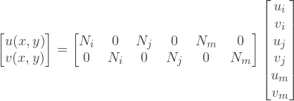
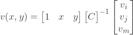
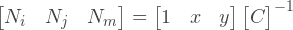
[N] (, ) . . , u v , , :
:
? , . -, , . :
f , :
:
, :
, :
, , :
, :
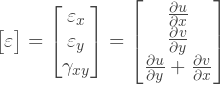
Knowing the displacement field, we can find the strain field on the relations of the theory of elasticity:
Now we can replace u and v , in the form of functions:
Or we can write the same in combined form:
The matrix on the right side, commonly referred to as a matrix in , the so-called gradient matrix.
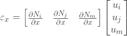
To find the matrix B , we must find all partial derivatives of the functions of the form:
In the case of a linear element, we see that the partial derivatives of the functions of the form are in fact constants, which will save us a lot of effort, as will be shown later. Multiplying the row vector with constants by the inverse matrix C we get:
Now we can calculate the B matrix. To build the matrix C, we first define the coordinate vectors of the nodes:
Eigen::Vector3f x, y; x << nodesX[nodesIds[0]], nodesX[nodesIds[1]], nodesX[nodesIds[2]]; y << nodesY[nodesIds[0]], nodesY[nodesIds[1]], nodesY[nodesIds[2]]; Then, we can build a matrix C of three rows:
Eigen::Matrix3f C; C << Eigen::Vector3f(1.0f, 1.0f, 1.0f), x, y; Then we compute the inverse matrix C and collect the matrix B:
Eigen::Matrix3f IC = C.inverse(); for (int i = 0; i < 3; i++) { B(0, 2 * i + 0) = IC(1, i); B(0, 2 * i + 1) = 0.0f; B(1, 2 * i + 0) = 0.0f; B(1, 2 * i + 1) = IC(2, i); B(2, 2 * i + 0) = IC(2, i); B(2, 2 * i + 1) = IC(1, i); } Transition to stress
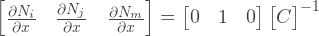
, D:
, , :
, , . . , , . , . , , .
, , . , : d[δ] e
, . , , , . , , , .
, :
- :
Or:
, :
, :
, , :
, . , , , :
, , . , :
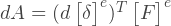
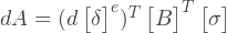
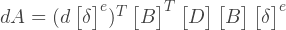
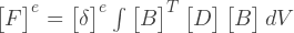
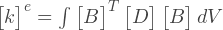
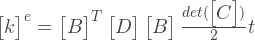
A — , t — . , :
, :
Eigen::Matrix<float, 6, 6> K = B.transpose() * D * B * C.determinant() / 2.0f; , . , : , 2 . , , , . , . , .
CalculateStiffnessMatrix :
void Element::CalculateStiffnessMatrix(const Eigen::Matrix3f& D, std::vector<Eigen::Triplet<float> >& triplets) { Eigen::Vector3f x, y; x << nodesX[nodesIds[0]], nodesX[nodesIds[1]], nodesX[nodesIds[2]]; y << nodesY[nodesIds[0]], nodesY[nodesIds[1]], nodesY[nodesIds[2]]; Eigen::Matrix3f C; C << Eigen::Vector3f(1.0f, 1.0f, 1.0f), x, y; Eigen::Matrix3f IC = C.inverse(); for (int i = 0; i < 3; i++) { B(0, 2 * i + 0) = IC(1, i); B(0, 2 * i + 1) = 0.0f; B(1, 2 * i + 0) = 0.0f; B(1, 2 * i + 1) = IC(2, i); B(2, 2 * i + 0) = IC(2, i); B(2, 2 * i + 1) = IC(1, i); } Eigen::Matrix<float, 6, 6> K = B.transpose() * D * B * C.determinant() / 2.0f; for (int i = 0; i < 3; i++) { for (int j = 0; j < 3; j++) { Eigen::Triplet<float> trplt11(2 * nodesIds[i] + 0, 2 * nodesIds[j] + 0, K(2 * i + 0, 2 * j + 0)); Eigen::Triplet<float> trplt12(2 * nodesIds[i] + 0, 2 * nodesIds[j] + 1, K(2 * i + 0, 2 * j + 1)); Eigen::Triplet<float> trplt21(2 * nodesIds[i] + 1, 2 * nodesIds[j] + 0, K(2 * i + 1, 2 * j + 0)); Eigen::Triplet<float> trplt22(2 * nodesIds[i] + 1, 2 * nodesIds[j] + 1, K(2 * i + 1, 2 * j + 1)); triplets.push_back(trplt11); triplets.push_back(trplt12); triplets.push_back(trplt21); triplets.push_back(trplt22); } } } , , Triplets . Triplet , . , , , — , — .
The resulting system of linear equations cannot be solved until we specify the fixings. Purely from a mechanical point of view, an unsecured system can make any large displacements, and under the action of external forces, it can even go into motion. Mathematically, this will lead to the fact that the resulting SLAE is not linearly independent, and therefore does not have a unique solution.
Moves of some nodes must be set to zero or to some predetermined value. In the simplest case, let's consider only the fixing of the nodes, without initial displacements. In fact, this means that we remove some equations from the system. But changing the number of equations of the system on the fly is not a trivial task. Instead, you can use the following trick.
Let's say we have the following system of equations:
To fix a node, the corresponding matrix element must be set to 1, and all elements in the row and column containing this element must be set to zero. There should also be no external forces acting on the fixed node in the direction in which the restriction is valid. An equation with this node will explicitly give a zero offset for this node, and the zeros in the corresponding column will exclude this offset from other equations. Let's say we want to fix the zero node in the direction of the x axis, and fix the first node in the direction of the y axis:
To perform this operation, we first define the indices of the equations that we are going to exclude from the SLAE. To do this, we loop through the list of assignments and collect the vector of indices. Then, going through all the nonzero elements of the stiffness matrix, we call the function SetConstraints . The following is the ApplyConstraints function :
void ApplyConstraints(Eigen::SparseMatrix<float>& K, const std::vector<Constraint>& constraints) { std::vector<int> indicesToConstraint; for (std::vector<Constraint>::const_iterator it = constraints.begin(); it != constraints.end(); ++it) { if (it->type & Constraint::UX) { indicesToConstraint.push_back(2 * it->node + 0); } if (it->type & Constraint::UY) { indicesToConstraint.push_back(2 * it->node + 1); } } for (int k = 0; k < K.outerSize(); ++k) { for (Eigen::SparseMatrix<float>::InnerIterator it(K, k); it; ++it) { for (std::vector<int>::iterator idit = indicesToConstraint.begin(); idit != indicesToConstraint.end(); ++idit) { SetConstraints(it, *idit); } } } } The SetConstraints function checks whether an element of the stiffness matrix is part of the excluded equation, and if so, it sets it equal to zero or one, depending on whether the element is on the diagonal or not:
void SetConstraints(Eigen::SparseMatrix<float>::InnerIterator& it, int index) { if (it.row() == index || it.col() == index) { it.valueRef() = it.row() == it.col() ? 1.0f : 0.0f; } } Further, we simply call ApplyConstraints and pass as its arguments a global stiffness matrix and a vector of constraints:
ApplyConstraints(globalK, constraints); SLAE solution and output
The Eigen library has various sparse linear equations solvers available, we will use SimplicialLDLT , which is a fast direct solver. For demonstration purposes, we will derive the initial stiffness matrix and load vector, and then output the result of the solution, the displacement vector.
std::cout << "Global stiffness matrix:\n"; std::cout << static_cast<const Eigen::SparseMatrixBase<Eigen::SparseMatrix<float> >& > (globalK) << std::endl; std::cout << "Loads vector:" << std::endl << loads << std::endl << std::endl; Eigen::SimplicialLDLT<Eigen::SparseMatrix<float> > solver(globalK); Eigen::VectorXf displacements = solver.solve(loads); std::cout << "Displacements vector:" << std::endl << displacements << std::endl; outfile << displacements << std::endl; Of course, the matrix output makes sense only for our test example, which contains only two elements.
Analysis of the result
As we have seen before, we can move from displacements to deformations and further to stresses:
However, we obtain a stress vector, which in theory of elasticity is generally a second-rank symmetric tensor:
As you know, the tensor elements directly depend on the coordinate system, however the physical state itself is of course independent. Therefore, for analysis, it is better to proceed as an invariant value, best of all, to a scalar one. Such an invariant is the von Mises stresses :
, - , . , , , .
, :
std::cout << "Stresses:" << std::endl; for (std::vector<Element>::iterator it = elements.begin(); it != elements.end(); ++it) { Eigen::Matrix<float, 6, 1> delta; delta << displacements.segment<2>(2 * it->nodesIds[0]), displacements.segment<2>(2 * it->nodesIds[1]), displacements.segment<2>(2 * it->nodesIds[2]); Eigen::Vector3f sigma = D * it->B * delta; float sigma_mises = sqrt(sigma[0] * sigma[0] - sigma[0] * sigma[1] + sigma[1] * sigma[1] + 3.0f * sigma[2] * sigma[2]); std::cout << sigma_mises << std::endl; outfile << sigma_mises << std::endl; } . , :
Global stiffness matrix: 1 0 0 0 0 0 0 0 0 1 0 0 0 0 0 0 0 0 1483.52 0 0 714.286 -384.615 -384.615 0 0 0 1 0 0 0 0 0 0 0 0 1483.52 0 -1098.9 -329.67 0 0 714.286 0 0 1483.52 -384.615 -384.615 0 0 -384.615 0 -1098.9 -384.615 1483.52 714.286 0 0 -384.615 0 -329.67 -384.615 714.286 1483.52 Loads vector: 0 0 0 0 0 1 0 1 Deformations vector: 0 0 -0.0003 0 -5.27106e-011 0.001 -0.0003 0.001 Stresses: 2 2 , , . , . x-, 0.0003, 0.3 y-, . , .
#include <Eigen/Dense> #include <Eigen/Sparse> #include <string> #include <vector> #include <iostream> #include <fstream> struct Element { void CalculateStiffnessMatrix(const Eigen::Matrix3f& D, std::vector<Eigen::Triplet<float> >& triplets); Eigen::Matrix<float, 3, 6> B; int nodesIds[3]; }; struct Constraint { enum Type { UX = 1 << 0, UY = 1 << 1, UXY = UX | UY }; int node; Type type; }; int nodesCount; Eigen::VectorXf nodesX; Eigen::VectorXf nodesY; Eigen::VectorXf loads; std::vector< Element > elements; std::vector< Constraint > constraints; void Element::CalculateStiffnessMatrix(const Eigen::Matrix3f& D, std::vector<Eigen::Triplet<float> >& triplets) { Eigen::Vector3f x, y; x << nodesX[nodesIds[0]], nodesX[nodesIds[1]], nodesX[nodesIds[2]]; y << nodesY[nodesIds[0]], nodesY[nodesIds[1]], nodesY[nodesIds[2]]; Eigen::Matrix3f C; C << Eigen::Vector3f(1.0f, 1.0f, 1.0f), x, y; Eigen::Matrix3f IC = C.inverse(); for (int i = 0; i < 3; i++) { B(0, 2 * i + 0) = IC(1, i); B(0, 2 * i + 1) = 0.0f; B(1, 2 * i + 0) = 0.0f; B(1, 2 * i + 1) = IC(2, i); B(2, 2 * i + 0) = IC(2, i); B(2, 2 * i + 1) = IC(1, i); } Eigen::Matrix<float, 6, 6> K = B.transpose() * D * B * C.determinant() / 2.0f; for (int i = 0; i < 3; i++) { for (int j = 0; j < 3; j++) { Eigen::Triplet<float> trplt11(2 * nodesIds[i] + 0, 2 * nodesIds[j] + 0, K(2 * i + 0, 2 * j + 0)); Eigen::Triplet<float> trplt12(2 * nodesIds[i] + 0, 2 * nodesIds[j] + 1, K(2 * i + 0, 2 * j + 1)); Eigen::Triplet<float> trplt21(2 * nodesIds[i] + 1, 2 * nodesIds[j] + 0, K(2 * i + 1, 2 * j + 0)); Eigen::Triplet<float> trplt22(2 * nodesIds[i] + 1, 2 * nodesIds[j] + 1, K(2 * i + 1, 2 * j + 1)); triplets.push_back(trplt11); triplets.push_back(trplt12); triplets.push_back(trplt21); triplets.push_back(trplt22); } } } void SetConstraints(Eigen::SparseMatrix<float>::InnerIterator& it, int index) { if (it.row() == index || it.col() == index) { it.valueRef() = it.row() == it.col() ? 1.0f : 0.0f; } } void ApplyConstraints(Eigen::SparseMatrix<float>& K, const std::vector<Constraint>& constraints) { std::vector<int> indicesToConstraint; for (std::vector<Constraint>::const_iterator it = constraints.begin(); it != constraints.end(); ++it) { if (it->type & Constraint::UX) { indicesToConstraint.push_back(2 * it->node + 0); } if (it->type & Constraint::UY) { indicesToConstraint.push_back(2 * it->node + 1); } } for (int k = 0; k < K.outerSize(); ++k) { for (Eigen::SparseMatrix<float>::InnerIterator it(K, k); it; ++it) { for (std::vector<int>::iterator idit = indicesToConstraint.begin(); idit != indicesToConstraint.end(); ++idit) { SetConstraints(it, *idit); } } } } int main(int argc, char *argv[]) { if ( argc != 3 ) { std::cout<<"usage: "<< argv[0] <<" <input file> <output file>\n"; return 1; } std::ifstream infile(argv[1]); std::ofstream outfile(argv[2]); float poissonRatio, youngModulus; infile >> poissonRatio >> youngModulus; Eigen::Matrix3f D; D << 1.0f, poissonRatio, 0.0f, poissonRatio, 1.0, 0.0f, 0.0f, 0.0f, (1.0f - poissonRatio) / 2.0f; D *= youngModulus / (1.0f - pow(poissonRatio, 2.0f)); infile >> nodesCount; nodesX.resize(nodesCount); nodesY.resize(nodesCount); for (int i = 0; i < nodesCount; ++i) { infile >> nodesX[i] >> nodesY[i]; } int elementCount; infile >> elementCount; for (int i = 0; i < elementCount; ++i) { Element element; infile >> element.nodesIds[0] >> element.nodesIds[1] >> element.nodesIds[2]; elements.push_back(element); } int constraintCount; infile >> constraintCount; for (int i = 0; i < constraintCount; ++i) { Constraint constraint; int type; infile >> constraint.node >> type; constraint.type = static_cast<Constraint::Type>(type); constraints.push_back(constraint); } loads.resize(2 * nodesCount); loads.setZero(); infile >> loadsCount; int loadsCount; for (int i = 0; i < loadsCount; ++i) { int node; float x, y; infile >> node >> x >> y; loads[2 * node + 0] = x; loads[2 * node + 1] = y; } std::vector<Eigen::Triplet<float> > triplets; for (std::vector<Element>::iterator it = elements.begin(); it != elements.end(); ++it) { it->CalculateStiffnessMatrix(D, triplets); } Eigen::SparseMatrix<float> globalK(2 * nodesCount, 2 * nodesCount); globalK.setFromTriplets(triplets.begin(), triplets.end()); ApplyConstraints(globalK, constraints); Eigen::SimplicialLDLT<Eigen::SparseMatrix<float> > solver(globalK); Eigen::VectorXf displacements = solver.solve(loads); outfile << displacements << std::endl; for (std::vector<Element>::iterator it = elements.begin(); it != elements.end(); ++it) { Eigen::Matrix<float, 6, 1> delta; delta << displacements.segment<2>(2 * it->nodesIds[0]), displacements.segment<2>(2 * it->nodesIds[1]), displacements.segment<2>(2 * it->nodesIds[2]); Eigen::Vector3f sigma = D * it->B * delta; float sigma_mises = sqrt(sigma[0] * sigma[0] - sigma[0] * sigma[1] + sigma[1] * sigma[1] + 3.0f * sigma[2] * sigma[2]); outfile << sigma_mises << std::endl; } return 0; } cloc :
------------------------------------------------------------------------------- Language files blank comment code ------------------------------------------------------------------------------- C++ 1 37 0 171 ------------------------------------------------------------------------------- , — 171 .
Some pictures
, python, . , PIL , . Abaqus , , .
:
, Abaqus . Abaqus ' . .
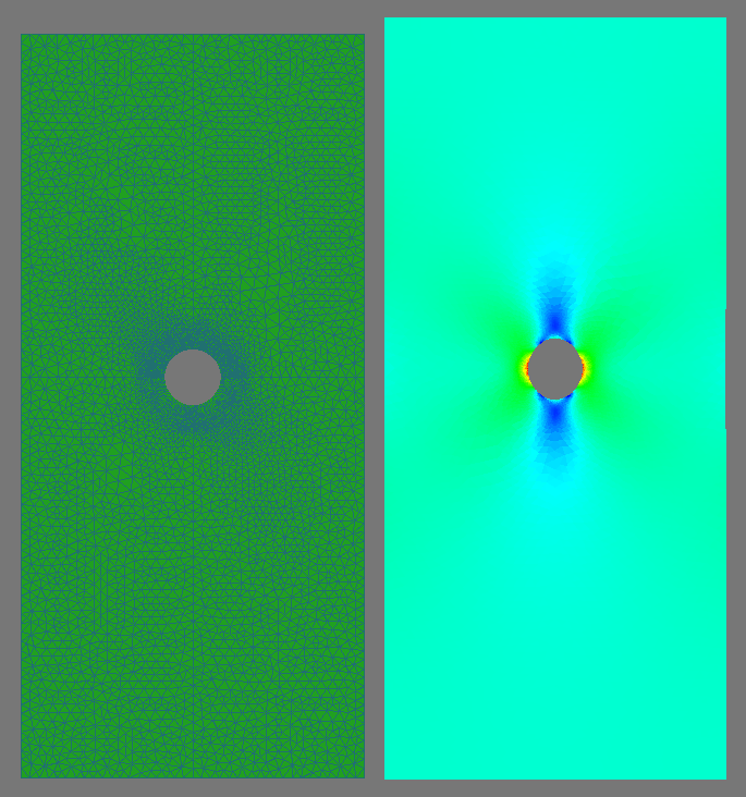
Here we see a strip with a hole, the bottom of which is fixed, and a tensile force is applied to the upper edge:
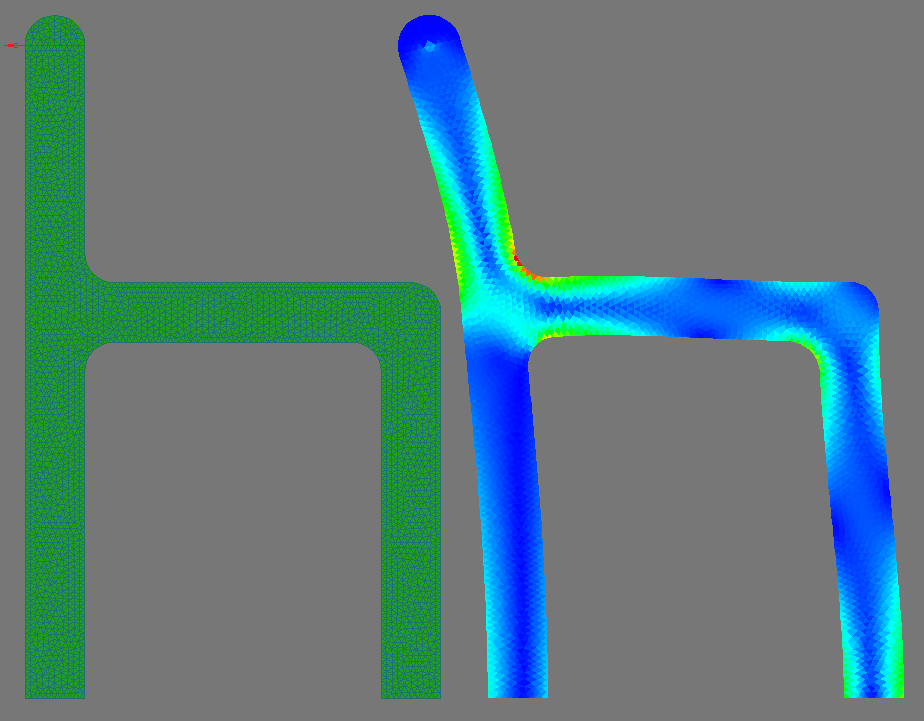
Abstract structural element, just for beauty. The bottom of the structure is fixed, and a concentrated force is applied on the upper protruding part, which I have already drawn on top of the picture:
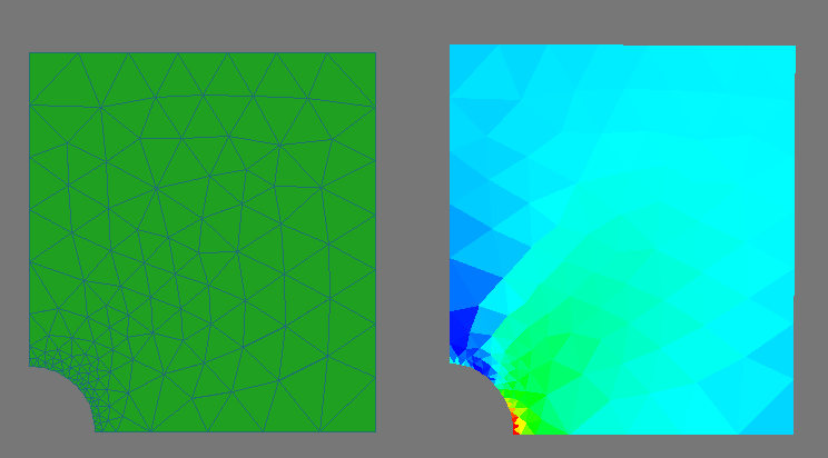
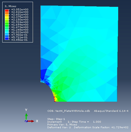
Another example with a strip with a hole, this time only a quarter of the structure is considered due to symmetry. The left border is fixed along the x axis, the lower one along the y axis. The maximum voltage received: 3.05152. This value, despite the coarseness of the grid (and perhaps because of it), is quite close to the theoretical value - 3.
The same problem, but solved in Abaqus. As you can see, the maximum voltage is 3.052, which fully coincides with our result. Such an exact coincidence, in principle, is not surprising, since in practice, it is difficult for a triangular element to do something in some way, so that the result is different. For elements of a higher order, unfortunately, such a 100% coincidence did not work out for me, which can be explained by different implementation of numerical integration.
All source code, including examples, is available on github .
What's left overs
Honestly, behind the scenes there are quite a lot. But the article turned out to be inflated, and so I think this can be stopped.
Not included (but wanted):
- . , . . , ( 2- 4- ), . , ( ).
- .
- , .
- - , . , .
- , , .
- , , , .
, , , MATLAB , ++. , , , .. . , , .
PS , , .
Source: https://habr.com/ru/post/271723/
All Articles