Neural network in 11 lines in Python

What is the article about

Personally, I learn best with a small, working code I can play with. In this tutorial, we will learn the error back-propagation algorithm using the example of a small neural network implemented in Python.

Give the code!

X = np.array([ [0,0,1],[0,1,1],[1,0,1],[1,1,1] ]) y = np.array([[0,1,1,0]]).T syn0 = 2*np.random.random((3,4)) - 1 syn1 = 2*np.random.random((4,1)) - 1 for j in xrange(60000): l1 = 1/(1+np.exp(-(np.dot(X,syn0)))) l2 = 1/(1+np.exp(-(np.dot(l1,syn1)))) l2_delta = (y - l2)*(l2*(1-l2)) l1_delta = l2_delta.dot(syn1.T) * (l1 * (1-l1)) syn1 += l1.T.dot(l2_delta) syn0 += XTdot(l1_delta) 

Too compressed? Let's break it down into simpler parts.

Part 1: A small toy neural network

A neural network that is trained through backpropagation attempts to use input data to predict the output.
')

   0 0 1 0 1 1 1 1 1 0 1 1 0 1 1 0 

Suppose we need to predict what the output column will look like based on the input data. This problem could be solved by calculating the statistical correspondence between them. And we would see that the left column correlates 100% with the output.

Backpropagation, in the simplest case, calculates similar statistics to create a model. Let's try.

Neural network in two layers

 import numpy as np #  def nonlin(x,deriv=False): if(deriv==True): return f(x)*(1-f(x)) return 1/(1+np.exp(-x)) #    X = np.array([ [0,0,1], [0,1,1], [1,0,1], [1,1,1] ]) #   y = np.array([[0,0,1,1]]).T #      np.random.seed(1) #       0 syn0 = 2*np.random.random((3,1)) - 1 for iter in xrange(10000): #   l0 = X l1 = nonlin(np.dot(l0,syn0)) #   ? l1_error = y - l1 #      #     l1 l1_delta = l1_error * nonlin(l1,True) # !!! #   syn0 += np.dot(l0.T,l1_delta) # !!! print "   :" print l1 

    : [[ 0.00966449] [ 0.00786506] [ 0.99358898] [ 0.99211957]] 

Variables and their descriptions.

X - matrix input data set; strings - training examples
y is the matrix of the output data set; strings - training examples
l0 is the first network layer defined by the input data
l1 - the second layer of the network, or hidden layer
syn0 - the first layer of the scale, Synapse 0, combines l0 with l1.
"*" - elementwise multiplication - two vectors of the same size multiply the corresponding values, and the output is a vector of the same size
"-" - elementwise subtraction of vectors
x.dot (y) - if x and y are vectors, then the output will be the scalar product. If these are matrices, then matrix multiplication will be obtained. If the matrix is ​​only one of them - this is the multiplication of the vector and the matrix.

And it works! I recommend before reading the explanations to play around a bit with the code and understand how it works. It should run just like it is, in ipython notebook. What you can tinker with in the code:

• compare l1 after the first iteration and after the last
• look at the nonlin function.
• see how l1_error changes
• parse line 36 - the main secret ingredients are collected here (marked !!!)
• parse line 39 - the entire network is preparing for this operation (marked !!!)

Let's sort the code by lines

 import numpy as np 

Imports numpy, a library of linear algebra. Our only dependency.

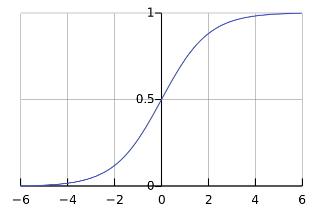
 def nonlin(x,deriv=False): 

Our nonlinearity. Specifically, this function creates a "sigmoid." It assigns any number to a value from 0 to 1 and converts numbers to probabilities, and also has several other properties useful for training neural networks.

 if(deriv==True): 

This function also can produce derived sigmoids (deriv = True). This is one of its useful properties. If the output of the function is the out variable, then the derivative will be out * (1-out). Effectively.

 X = np.array([ [0,0,1], … 

Initialization of the input data array in the form of a numpy-matrix. Each line is a training example. Columns are input nodes. We have 3 input nodes in the network and 4 training examples.

 y = np.array([[0,0,1,1]]).T 

Initializes the output. ".T" is the transfer function. After the transfer, the matrix y has 4 rows with one column. As in the case of input data, each row is a training example, and each column (in our case one) is an output node. At the network, it turns out, 3 inputs and 1 output.

 np.random.seed(1) 

Due to this, the random distribution will be the same each time. This will allow us to more easily track the network after making changes to the code.

 syn0 = 2*np.random.random((3,1)) – 1 

Matrix weights network. syn0 means "synapse zero". Since we have only two layers, input and output, we need one matrix of weights, which will connect them. Its dimension is (3, 1), since we have 3 inputs and 1 output. In other words, l0 has size 3, and l1 is 1. Since we connect all nodes in l0 with all nodes l1, we need a matrix of dimension (3, 1).

Notice that it is initialized randomly, and the average value is zero. Behind this is quite a complex theory. For now, just accept this as a recommendation. Also note that our neural network is this very matrix. We have “layers” of l0 and l1, but they are temporary values ​​based on a data set. We do not store them. All training is stored in syn0.

 for iter in xrange(10000): 

This is where the main workout code for the network begins. The code loop repeats many times and optimizes the network for the data set.

 l0 = X 

The first layer, l0, is just data. X contains 4 training examples. We will process them all at once - this is called full batch training. In total, we have 4 different lines of l0, but they can be thought of as one training example - at this stage it does not matter (you could load them 1000 or 10,000 without any changes in the code).

 l1 = nonlin(np.dot(l0,syn0)) 

This is a prediction step. We allow the network to try to predict output based on input. Then we will see how she does it so that you can tweak her in the direction of improvement.

The line contains two steps. The first makes the matrix multiplication l0 and syn0. The second transmits the output through sigmoid. They have the following dimensions:

 (4 x 3) dot (3 x 1) = (4 x 1) 

Matrix multiplications require that the dimension equations in the middle coincide. The final matrix has the number of rows, as in the first, and the columns - as in the second.

We downloaded 4 training examples, and got 4 guesses (4x1 matrix). Each pin corresponds to a guess of the network for a given input.

 l1_error = y - l1 

Since l1 contains guesses, we can compare their difference with reality, subtracting its l1 from the correct answer y. l1_error is a vector of positive and negative numbers characterizing the “miss” of the network.

  l1_delta = l1_error * nonlin(l1,True) 

And here is the secret ingredient. This line must be disassembled in parts.

First part: derivative

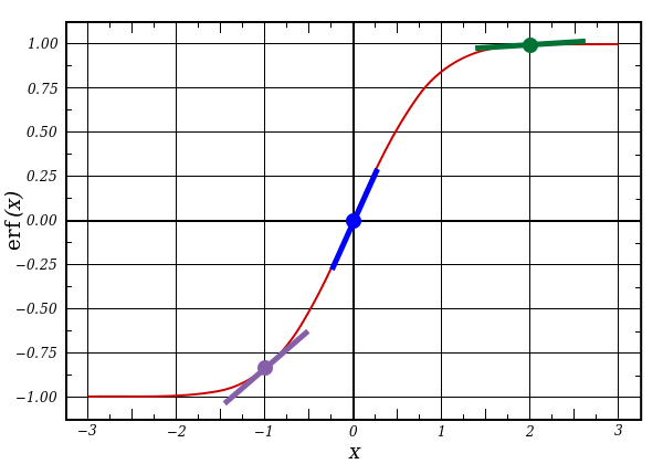
 nonlin(l1,True) 

l1 represents these three points, and the code gives the slope of the lines shown below. Note that for large values ​​like x = 2.0 (green dot) and very small ones, like x = -1.0 (purple), the lines have a slight bias. The largest angle of the point is x = 0 (blue). It is of great importance. Also note that all derivatives are in the range of 0 to 1.



Full Expression: Error Weighted Derivative

 l1_delta = l1_error * nonlin(l1,True) 

Mathematically there are more accurate ways, but in our case this one is also suitable. l1_error is a matrix (4,1). nonlin (l1, true) returns a matrix (4,1). Here we multiply them element by element, and at the output we also get the matrix (4,1), l1_delta.

By multiplying the derivatives by errors, we reduce the prediction errors made with high confidence. If the slope of the line was small, then the network contains either a very large or a very small value. If the guess in the network is close to zero (x = 0, y = 0.5), then it is not particularly sure. We update these uncertain predictions and leave predictions alone with high confidence, multiplying them by values ​​close to zero.

 syn0 += np.dot(l0.T,l1_delta) 

We are ready to update the network. Consider one training example. In it, we will update the weight. Update the leftmost weight (9.5)

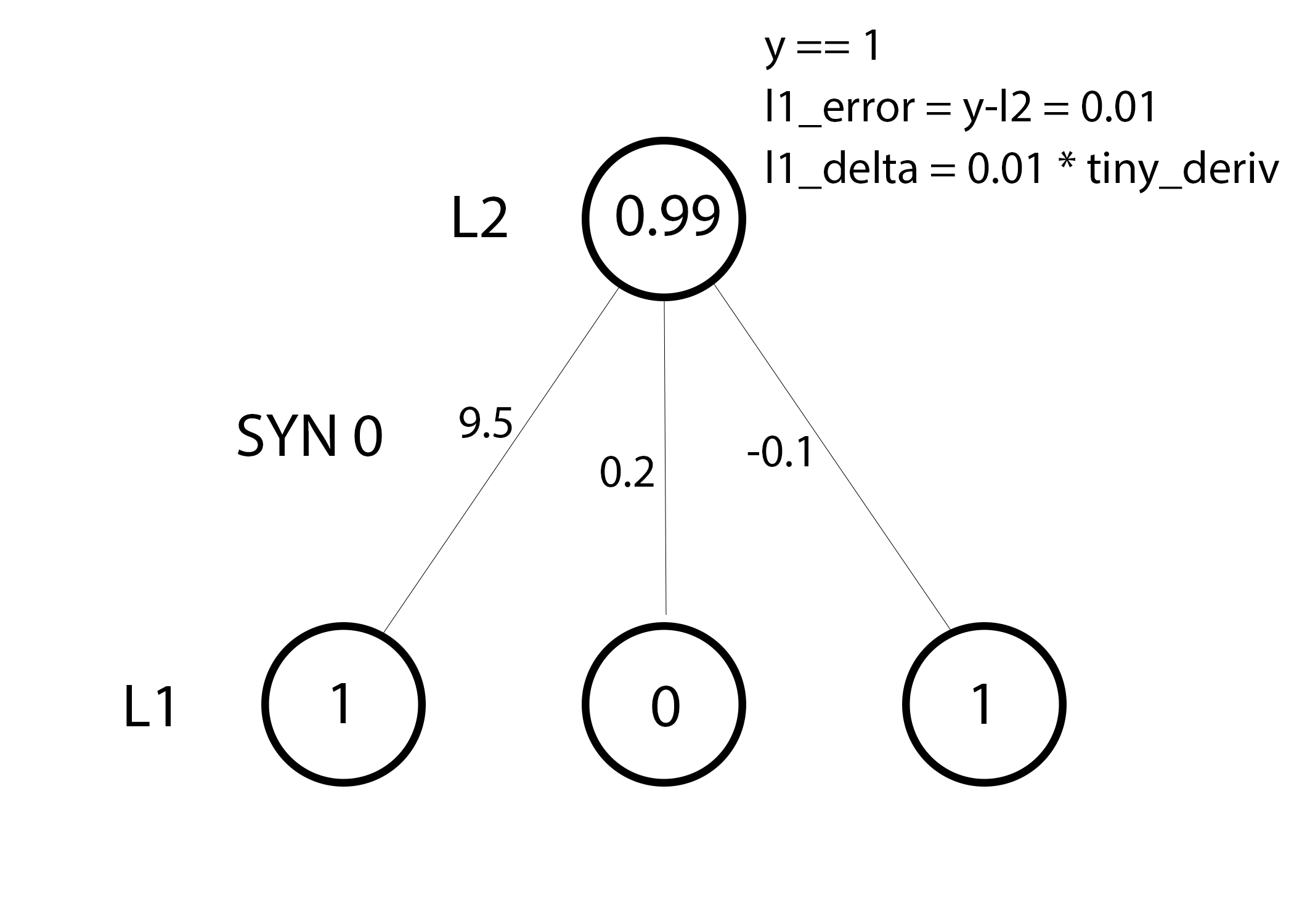
 weight_update = input_value * l1_delta 

For the extreme left weight, this will be 1.0 * l1_delta. Presumably, this will only slightly increase 9.5. Why? Since the prediction was already quite confident, and the predictions were almost correct. A small error and a slight slope of the line mean a very small update.



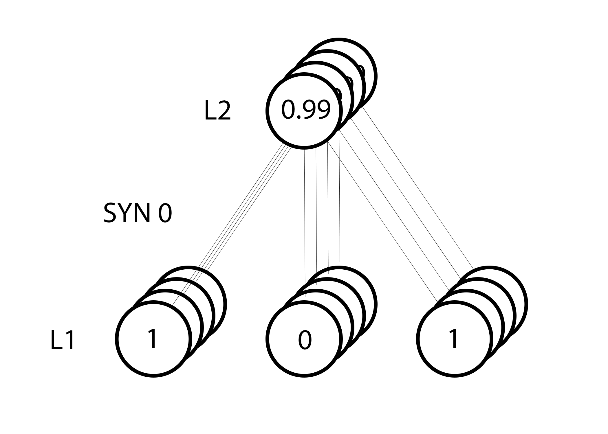
But since we are doing group training, we repeat the above step for all four training examples. So this looks very much like the image above. So what does our line do? It calculates the weights updates for each weight, for each training example, summarizes them and updates all weights - all in one line.

After watching the network update, let's return to our training data. When both the input and output are 1, we increase the weight between them. When the input is 1 and the output is 0, we reduce the weight.

   0 0 1 0 1 1 1 1 1 0 1 1 0 1 1 0 

Thus, in our four training examples below, the weight of the first input relative to the output will constantly increase or remain constant, and the other two weights will increase and decrease depending on the examples. This effect contributes to network training based on the correlation of input and output data.

Part 2: the task is more difficult

   0 0 1 0 0 1 1 1 1 0 1 1 1 1 1 0 

Let's try to predict the output based on the three input data columns. None of the input columns is 100% correlated with the output. The third column is not connected with anything at all, since it contains units all the way. However, here you can see the scheme - if one of the first two columns (but not both) contains 1, then the result will also be equal to 1.

This is a non-linear scheme, since there is no direct correspondence of one-to-one columns. The match is based on a combination of input data, columns 1 and 2.

Interestingly, pattern recognition is a very similar task. If you have 100 pictures of the same size, on which bicycles and smoking pipes are depicted, the presence of certain pixels on them in certain places does not directly correlate with the presence of a bicycle or tube on the image. Statistically, their color may seem random. But some combinations of pixels are not random - those that form the image of a bicycle (or tube).

Strategy

To combine pixels into something that can have a one-to-one correspondence with the output, you need to add another layer. The first layer combines the input, the second one assigns the matching to the output, using the input data of the first layer as input. Pay attention to the table.

  (l0)   (l1)  (l2) 0 0 1 0.1 0.2 0.5 0.2 0 0 1 1 0.2 0.6 0.7 0.1 1 1 0 1 0.3 0.2 0.3 0.9 1 1 1 1 0.2 0.1 0.3 0.8 0 

By randomly assigning weights, we get the hidden values ​​for layer # 1. Interestingly, the second column of the hidden scales already has a slight correlation with the exit. Not perfect, but there is. And this is also an important part of the network training process. Training will only enhance this correlation. It will update syn1 to match its output, and syn0 to better receive data from the input.

Neural network in three layers

 import numpy as np def nonlin(x,deriv=False): if(deriv==True): return f(x)*(1-f(x)) return 1/(1+np.exp(-x)) X = np.array([[0,0,1], [0,1,1], [1,0,1], [1,1,1]]) y = np.array([[0], [1], [1], [0]]) np.random.seed(1) #   ,   - 0 syn0 = 2*np.random.random((3,4)) - 1 syn1 = 2*np.random.random((4,1)) - 1 for j in xrange(60000): #     0, 1  2 l0 = X l1 = nonlin(np.dot(l0,syn0)) l2 = nonlin(np.dot(l1,syn1)) #       ? l2_error = y - l2 if (j% 10000) == 0: print "Error:" + str(np.mean(np.abs(l2_error))) #     ? #      ,       l2_delta = l2_error*nonlin(l2,deriv=True) #    l1     l2? l1_error = l2_delta.dot(syn1.T) #     ,    l1? #      ,       l1_delta = l1_error * nonlin(l1,deriv=True) syn1 += l1.T.dot(l2_delta) syn0 += l0.T.dot(l1_delta) 

 Error:0.496410031903 Error:0.00858452565325 Error:0.00578945986251 Error:0.00462917677677 Error:0.00395876528027 Error:0.00351012256786 

Variables and their descriptions

X - matrix input data set; strings - training examples
y is the matrix of the output data set; strings - training examples
l0 is the first network layer defined by the input data
l1 - the second layer of the network, or hidden layer
l2 is the final layer, this is our hypothesis. As the workout should approach the correct answer
syn0 - the first layer of the scale, Synapse 0, combines l0 with l1.
syn1 - the second layer of the scale, Synapse 1, combines l1 with l2.
l2_error - network miss in quantitative terms
l2_delta - network error, depending on the confidence of the prediction. Almost coincides with the error, except for confident predictions
l1_error - weighing l2_delta with weights from syn1, we calculate the error in the middle / hidden layer
l1_delta - network errors from l1, scalable according to the conviction of predictions. Almost identical to l1_error, except for confident predictions

The code should be clear enough - it is just the previous implementation of the network, folded in two layers one above the other. The output of the first layer l1 is the input of the second layer. Something new is only in the next line.

 l1_error = l2_delta.dot(syn1.T) 

Uses errors weighted by prediction confidence from l2 to calculate the error for l1. We get, we can say, an error weighted by contributions - we calculate the contribution to the errors in l2 made by the values ​​in the nodes l1. This step is called back propagation of errors. Then we update syn0 using the same algorithm as in the two-layer neural network version.