Machine learning as a method of analyzing the microstructure of the market and its application in high-frequency trading

In this article, we will look at how to use machine learning in high-frequency trading (HFT) and analyzing microstructural data. Machine learning is a wonderful section of computer science that uses models and methods from statistics, theory of algorithms, the theory of computational complexity, artificial intelligence, control theory, and a huge number of other disciplines. The main object of the study of machine learning are effective algorithms that allow you to create good predictive models based on large data sets - this is why it is so well suited for solving high-frequency trading problems: making deals and calculating the alpha indicator.

Since the phenomenon of “high-frequency trading” appeared quite recently, there are few works devoted to the use of machine learning in this field. However, we will consider three areas of its applicability:

1. Optimization of the process of making deals using reinforced learning;
2. Prediction of price changes based on the state of the stock exchange;
3. Optimization of the transaction process in dark pools based on the study of incomplete data.

Optimizing the process of making deals using reinforced learning

Let's consider the possibility of using machine learning to solve the most fundamental algorithmic trading problem - optimizing the process of concluding transactions. In the simplest case, the problem is determined by the stock of shares, say, AAPL, their number V, and the time or number of steps T. Thus, we must buy a certain number of shares V in T steps, minimizing the cost of the purchase.
')
The basic pricing algorithms, the weighted average volume, compare their current state (v; t) with the volume of shares, which must be acquired by step t, based on historical indicators of the stake of interest to us (the values ​​of the indicators may vary depending on the time of day and time of year ). If the indicator v tells us that we are behind the schedule, then we should start trading more aggressively and more often buy stocks at the price of the seller. If we are ahead of the schedule, then we can trade more passively, waiting for the price to improve. Such comparisons are carried out continuously or at certain intervals, allowing us to adjust to the schedule and current conditions on the exchange.

Training with reinforcements takes its beginning deep in control theory and is a machine learning subsection developed specifically for studying dynamic instructions. We omit the technical details, however, we describe the main steps:

1. Determining the state of the environment (usually limited), whose elements are changing conditions, depending on which procedure is chosen. In our case, the medium has two variables (v; t), as well as other components and features that describe the state of the stock exchange.
2. Defining a set of actions for each state. In our case, we will set a limit on orders for the remaining volume of shares (variable price).
3. Definition of the model of the impact that our decisions have in the form of the probability of execution under certain conditions, which is formed on the basis of historical data.
4. Determination of the cost function, reflecting the expected or average income when making a certain decision at a given point in time.
5. Algorithms for the study of optimal rules - the transition from states to actions - minimizing the empirical value of shares (the cost of their purchase) on the basis of training data.
6. Verification of the studied sequence of actions by assessing its performance outside the sample.

The potential of such a method can be observed in graphs (Figure 1). The graph compares the performance of a one-time strategy and algorithms studied using reinforcement training. One-time strategies at the beginning of the trading period fix the size of the limit of orders at a certain value p for the entire target volume V and do not change it throughout all T steps. At the end of the trading period, if the entire volume V was not purchased, the market order is given on condition that the target volume is reached. To normalize price differences for all blocks of shares, we measure performance by estimating the difference between the average amount paid (per share) and the average point of the spread at the beginning of the trading period - the smaller it is (the higher the average point of the spread), the better.



Figure 1 - One-time method performance on the test set (black left column) and learning performance with reinforcement (gray and white columns) on AMZN, NVDA and QCOM shares. The x-axis shows the target volume of shares and the period; the target volume is divided into I levels, and the period is divided into T discrete steps, uniformly distributed in time

So far, we practically did not use microstructural information and did not reconstruct the stock exchange glass - we only determined the purchase price and estimated its impact on the quotes glass. Machine learning allows you to improve performance if you pass more information to the algorithm. What variables related to the stock exchange can we use? Here are a few of them:

1. Bid-ask spread is a value that reflects the difference between the price of the buyer (bid) and the price of the seller (ask) in the current stock exchange;
2. The imbalance of bid / ask volumes is an amount equal to the number of purchased shares minus sold shares in current stock markets;
3. The transaction volume is a value that describes the number of shares purchased in the last 15 seconds, minus the number of shares sold during the same time period;
4. The cost of executing a market order at the moment is the price we pay for the purchase of the remaining share of shares by placing a market order.

We conducted a series of similar experiments in our initial state (v; t), using the characteristics of the stock exchange described above. The results obtained are summarized in table 1.

Table 1 - Reduced distribution costs, with the addition of new features

Signs of	Reduced handling costs
Bid-ask spread	7.97%
Imbalance bid / ask volumes	0.13%
Volume transactions	2.81%
Cost of Market Order Execution currently	4.26%
All signs immediately	12.85%

Three of the four signs resulted in significant improvements; imbalance bid / ask volumes had the least impact. The last row of the table reflects the increase in performance when using all signs at the same time - it is almost 13%.

Prediction of price changes based on the stock market state

It is worth noting that in the previous section we did not take into account many signs directly affecting the recent directional movements in the price of execution, which may be very important. Therefore, in the following experiments we used:

1. Bid-ask spread - used in the previous paragraph;
2. Price is a sign that reflects recent directional movements in execution prices;
3. The smart price is the average between the bid price and the bid price, weighted according to the inverse of their volume;
4. A trading indicator is a sign indicating how often buyers and sellers “crossed the spread”;
5. Imbalance bid / ask volumes - used in the previous paragraph;
6. Transaction amount - used in the previous paragraph.

In the first series of experiments, a short ten-second time interval was considered. It is important to note that buying or selling at an average price assumes that one of the two actions is always profitable: buying and then selling if the average price has increased, and vice versa if the price has fallen. In the real world, this approach does not work, so we will describe the methodology as follows:

1. For each of the 19 items, the stock exchange was restructured based on historical data;
2. For each trading opportunity, the current state of the stock exchange and the profitability of both actions (buy / sell or sell / buy) were evaluated. The results were recorded in the table of the stock exchange simulator, where the average point displacement was calculated;
3. For each item, 2008 data was used as training data. A function was calculated that determines which of the actions for a given ~ x state leads to the greatest performance increase;
4. Testing the principles studied for each item was conducted using the 2009 data set. For each state ~ x, the corresponding action learned by the algorithm was applied, after which the performance was calculated.

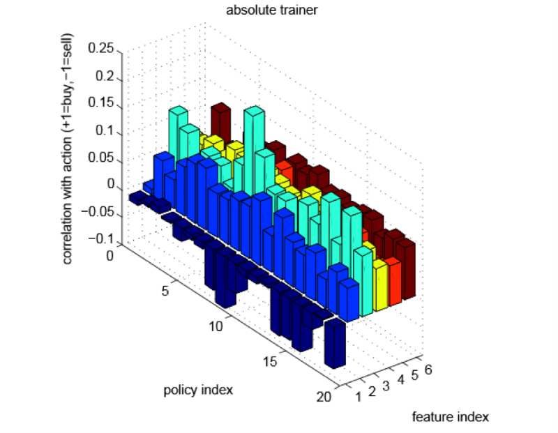
In Figure 2, for each of the 19 rules and each of the six signs, there is a bar showing the relationship between the value of the trait and the studied action. We agreed that the value +1 means buy and sell, and -1 means buy and sell. As in the last section, we see that the numerical values ​​of the correlation strongly depend on the chosen name.



Figure 2 - Correlation between the values ​​of attributes and the measures studied. Here, 1 is the bid-ask spread, 2 is the price, 3 is the “smart” price, 4 is the trade indicator, 5 is the bid / ask volume imbalance, 6 is the transaction volume

The image shows that we studied the strategies based on the moment: for each of the signs with directional information (price, smart price, trading indicator, bid / ask volume imbalance and transaction volume), high values ​​correspond to a higher purchase frequency in studied rules.



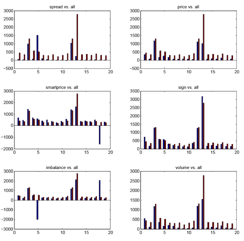
Figure 3 - graphics for each of the six signs

Figure 3 shows the graphs for each of the six features. The red bars are the same everywhere and show the profitability of the test set of rules learned for each of the 19 items, where all 6 signs were used. The blue bars show the profitability of the test set of rules learned for each of the 19 items, but using only one feature. From here we can draw conclusions:

1. The most advantageous to use immediately 6 signs;
2. The “smart” price makes the greatest contribution to profitability. It often happens that its use leads to a better result than using all six signs;
3. Spread is the most useless sign, but for individual items it turns out to be the most profitable.

Machine learning and smart systems routing applications in dark pools

The methodology of machine learning is applicable to newly-born areas that have less rich data volumes and new, unexplored mechanisms. Let's look at the application of machine learning to solve the problem of routing applications in dark pools.

Dark pools were initially viewed as locations for transactions where liquidity matters most. With sufficient liquidity, you can easily pay the "current price".

We assume that we have n separate dark pools available. These pools are able to provide different liquidity profiles for a certain block of shares - for example, in one pool it is better to quickly carry out small orders, and the other brings greater profitability from fulfilling large orders.

We assume that is a probability distribution describing the range of values ​​with non-negative integers. We assume that when confirming an order for shares for pool i, a random variable is chosen on the basis. represents stocks available on the other side of the market (stocks available for purchase, provided that we sell, or for sale if we buy) at the time of confirmation of the order. The problem of routing applications in dark pools can be formalized as follows: we have a given amount of V shares that we want to buy; How do we divide V into subsets for n dark pools so that, while maximizing the number of shares purchased?

Figure 4 shows what the real distribution of liquidity looks like. Shown here are the subsets and data used to conduct DELL stock purchase and sale transactions in the American dark pool.



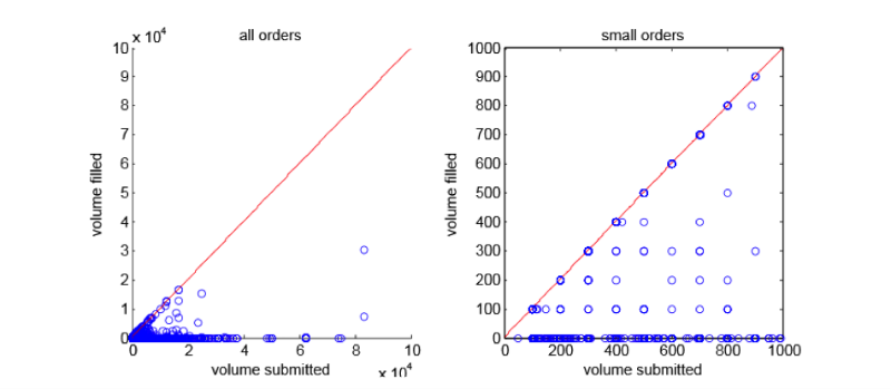
Figure 4 - Distribution of liquidity for DELL shares

The problem of learning the intelligent application routing system arises because we do not have enough knowledge about the probability distribution - we must study approximations based on our own data on applications. The details of the algorithm will remain outside the scope of this article, but, if we describe them in general terms, then:

1. The algorithm takes a certain approximation for each unknown liquidity distribution. Prior to the algorithm, all approximations take default values.
2. We use the Kaplan-Meier approximation, which estimates the similarity of closed data.
3. For each V, the algorithm considers the distribution of approximations to be true and selects the placements according to the greedy algorithm applied to the approximations Pi.

With the receipt of fresh business data, you can update the approximate distributions and repeat the process for the next target volume of shares.



Figure 5 - Performance curves of our learning algorithm (red) and simple adaptive heuristic algorithm (blue). Black marks uniform placement, and green is perfect.

Some experimental estimates of the performance of the algorithm are presented in Figure 5. Here are simulations using incomplete operational data for US dark pools. Each graph shows the performance change of our learning algorithm.

Conclusion

In this article, we introduced you to the possibilities of machine learning in the field of high-frequency trading and the microstructure of the market, as well as obstacles in its path. We do not believe that machine learning should be used according to the “black box” principle or look for any “amazing” trading strategies with it.

In each of the cases examined, the learning outcome did not produce results radically different from the general concepts of the problems under consideration from the point of view of economics and the theory of markets - the point of using machine learning was to quantitatively optimize these qualitative strategies. If this approach is applied carefully and in place, it can become a powerful and well-scalable tool that efficiently works with a huge amount of data currently available on the market microstructure.