Titanic on Kaggle: you do not finish reading this post until the end
Hi, Habr!

# {Data Science for newbies}
My name is Gleb Morozov, we are already familiar with the previous articles. Due to numerous requests, I continue to describe the experience of my participation in educational projects of MLClass.ru (by the way, who have not had time - you can still get the materials of past courses before the end - this is probably the shortest and most practical course in data analysis that you can imagine) .
This paper describes my attempt to create a model for predicting the surviving passengers of the Titanic. The main task is training in the use of tools used in Data Science for data analysis and presentation of research results, so this article will be very, very long . The focus is on exploratory research and on the creation and selection of predictors ( feature engineering ). The model is created as part of the Titanic: Machine Learning from Disaster competition on the Kaggle website. In my work I will use the language "R".
If you trust Wikipedia, then Titanic collided with an iceberg at 11:40 pm ship time, when the vast majority of passengers and ship crew were in their cabins. Accordingly, the location of the cabins may have had an impact on the likelihood of survival, since passengers of the lower decks, first, later learned about the collision and, accordingly, had less time to get to the upper deck. And, secondly, they naturally had to get out of the ship’s premises longer. Below are the schemes of the Titanic, indicating the decks and rooms.
')


The Titanic was a British ship, and according to the laws of Britain, the number of lifeboats that corresponded to the vessel’s displacement and not the passenger capacity had to be on the ship. Titanic formally met these requirements and had 20 boats (14 with a capacity of 65 people, 2 - 40 people, 4 - 47 people), which were designed to load 1178 people, just 2208 people on Titanic. Thus, knowing that there would not be enough boats for everyone, the captain of the Titanic Smith gave, after a collision with an iceberg, an order to take on boats only women and children. However, team members did not always follow him.
Kaggle provides data as two files in csv format:
To get the data in R, I use the read_csv function from the readr package. In comparison with the basic functions, this package provides a number of advantages, in particular: higher speed and clear names of parameters.
Let's see what we got:
I believe that research data analysis is one of the most important parts of Data Scientist's work, because, apart from directly transforming “raw” data into ready-made models, often during this process you can see hidden dependencies, thanks to which the most accurate models are obtained.
First, look at the missing data. In the data provided, a part of the missing information was marked with the symbol NA and, when loaded, were converted to the special symbol NA by default. But among symbolic variables there are many passengers with missing variables that were not marked. Check their availability using the capabilities of the packages magrittr and dplyr
Replace the blanks with NA, using the recode function from the car package.
For a graphical representation, it is convenient to use the missmap function from the package for working with missing Amelia data.

Thus, about 20% of the data in the Age variable and almost 80% in Cabin are missing. And if with the age of the passengers it is possible to make a reasonable replacement of the missing values, due to their small share, then it is unlikely to do something with the cabins, because Missing values are significantly more than filled. Missing Values in the Embarked Tag
We will return to the missing values later, but for now let's see what information can be extracted from the data that we have. I remind you that the main task is to determine the variables that affect the probability of surviving a Titanic crash. Let's try to get initial ideas about these dependencies using simple graphs.

Already it is possible to draw the first conclusions:
In general, we can already say that the main factors of the model will be the floor of the passenger (remember the order of the captain, about which I wrote earlier) and the location of the cabin.
Let's go back to the missing values for a while. From the schedule Distribution of passengers at the point of departure it is obvious that most of the passengers went from Southampton, respectively, you can safely replace 2 NA with this value
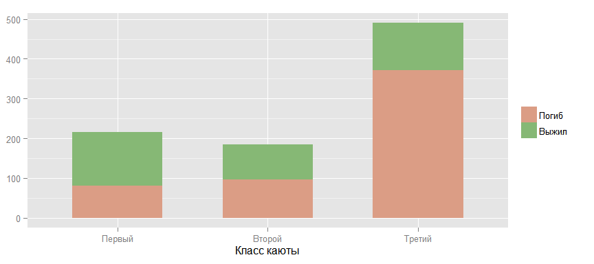
Now take a closer look at the relationship between the probability of survival and other factors. The following graph confirms the theory that the higher the passenger cabin class, the greater the chances of survival. (By "higher", "I mean the reverse order, because the first class is higher than the second and, especially, the third.)
Compare the chances of survival in men and women. The data confirm the theory expressed earlier.

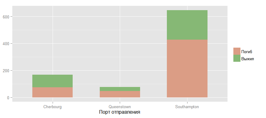
Now let's take a look at the chances of surviving passengers from various ports of departure.
It seems that there is some kind of connection, but I think that this is most likely due to the distribution of passengers of different classes between these ports, which is confirmed by the following graph.

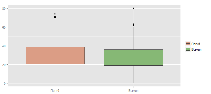
You can also test the hypothesis that younger people survive, because they move faster, swim better, etc.
As you can see, an obvious dependency is not visible here.
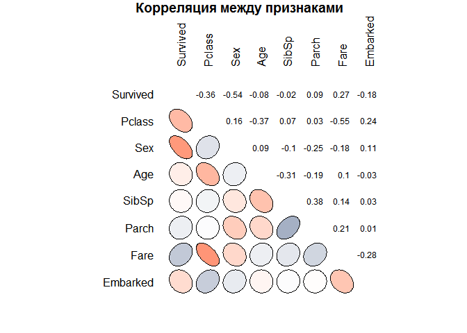
Now, with the help of another type of graph, let's look at the presence of possible statistical relationships between the features of objects. You can make preliminary conclusions that confirm the thoughts expressed earlier. In particular, that the chances of survival decrease with the growth of the class and age is a very weak symptom for building a model. You can also find other patterns. There is a negative correlation between age and class, which is most likely due to more aged passengers more often could afford a more expensive cabin. In addition, the ticket price and class are closely related (high correlation coefficient), which is quite expected.
Let's go back to the missing values in the data. One of the usual ways to deal with them is to replace them with an average of the available values of the same trait. For example, 177 missed from the sign Age can be replaced by 29.7
I have already successfully applied this method earlier with the Embarked sign, but there were only two replacements, and here - 177, which is more than 20% of all available data on this sign. Therefore, it is worth finding a more accurate way to replace.
One of the possible options is to take the average, but depending on the class of the cabin, because if you look at the chart below, this relationship is possible. And, if you think about it, such an assumption is intuitively clear: the older a person is, the higher his probable well-being and, accordingly, the higher level of comfort that he can afford. Thus, it is possible to replace the missing value for a passenger, for example, from the third class, with the average age for this class, which will already be a great progress compared to just the average for all passengers.
But let's turn to another of the possible options for replacing the missing values for the Age attribute. If you look at the values of the Name attribute, you can notice an interesting feature.
The name of each passenger is built one pattern each time: “Last Name, Gonorato. Name". The appeal of the Master in the 19th century was applied to male children, respectively, this can be used to single out narrower and more precise groups by age. And Miss was applied to unmarried women, but in the 19th century, in the overwhelming majority, only young girls and girls were unmarried. In order to use this dependency we will create a new Title attribute.
Now we define titles, among owners of which there is at least one with absent age.
And we will replace. To do this, create a function and apply it to the attribute Age.
If you pay attention to the sign of Fare (ticket price), you can see that there are tickets with zero cost.
The first explanation that comes to mind is the children, but if you look at the other signs of these passengers, this assumption turns out to be false.
Therefore, I think it would be logical to replace the zero values with the average values for the class using the already used impute.mean function.
The Title attribute, introduced to replace missing values in the Age attribute, gives us additional information about the passenger field, its nobility (for example, Don and Sir) and the priority in accessing the lifeboats. Therefore, this feature must be left when building a model. In total, we have 17 values of this attribute. The following graph shows their relationship with age.

But many of the values, as I believe, can be combined into 5 groups: Aristocratic, Mr, Mrs, Miss and Master, since merged titles belong in fact to one or related groups.

Let's introduce such an indicator as Survival Percentage and look at its dependence on the groups that turned out at the previous stage.

In order to get a good idea of the relationship between the signs is better than the graphics, as I think nothing has yet been invented. For example, according to the following graph, it is clearly seen that the main groups of survivors are women of the first and second class of all ages. And among the men, all the boys younger than 15 years old survived except the third class of service and a small proportion of older men and mostly from the first class.

Now look at the information that can be obtained from the number of relatives on the ship.

It is very likely that survival is negatively affected by the absence of relatives as well as a large number.
We introduce such a feature as Family, i.e. the number of relatives on board the ship and look at the effect on survival.
And also in the context of the sexes of passengers.

The graph shows that for a woman a small number of relatives significantly increases the likelihood of survival. The statistical significance of this dependence should be checked, but I think that the attribute should be left and to look at its influence when creating the model. It is also possible that such a binary sign as “Having relatives on board” will make sense.

At first glance, it seems that the presence of relatives increases the likelihood of survival, but if you look at the relationship in terms of classes and gender, the picture changes.
For a man in the second grade, relatives increase survival, but for a woman in the third grade, the situation is reversed.
From the sign of Cabin, i.e. cabin numbers occupied by the passenger, it would be possible to extract the deck number (this is the letter in the room) and on which board the cabin was (if the last digit of the number is odd, then this is the port side, and, accordingly, vice versa), but since only 20% of passengers have cabin numbers in the data, I do not think that this will significantly affect the accuracy of the model. Much more interesting, in my opinion, will be information about the availability of this number. The first-class cabin numbers became known from the list that was found on the body of the steward Herbert Cave, no further official information was preserved, respectively, it can be concluded that if the passenger room number of the second or third class is known, then he survived. Therefore, as with relatives, we will look at survival depending on the availability of a cabin room as a whole for all passengers and in a section by class and sex.


Obviously, the assumption was confirmed, especially for male passengers.
To summarize all the research work that has been done:
Now select from the data those signs that we will use when creating the model.
And the last schedule in this part of the work.

Prepare data for correct use in the process models.
In this paper, I will use the caret package, which has absorbed most of the well-known models of machine learning and provides a convenient interface for their practical use. Despite the fact that we have a test sample provided by the Kaggle site, we still need to split the training sample into two parts. On one of which we will train the model, and on the other, we will evaluate its quality before applying it to a competitive sample. I chose an 80/20 split.
Let's start with the simplest classification model - logistic regression. To evaluate the model, we will use the residual deviance statistics or residual deviation, which indirectly corresponds to the variance in the data, which is unexplained after the model has been applied. Null deviance or null deviance is the deviation of the “empty” model, which does not include any parameters other than beta0. Accordingly, the smaller the deviation of residuals in relation to the null deviance - the better the model. In the future, to compare different models, AUC statistics or the area under the ROC curve will be used.To correctly estimate this parameter, it will be estimated using a tenfold cross-validation (10-fold cross-validation (CV)) with the sample split into 10 parts.
So the first model is logistic regression. Predictors initially present in the data provided are selected as features.
The model already shows good performance in reducing deviance by 950-613 = 337 points compared to the “empty” model. Now we will try to improve this indicator by entering those new features that were added earlier.
, , , . , ROC, , p-value , , , . . isFamily, .. Family . , . Title.
, .., , .
And we got a significant leap as a model. At this stage, we’ll stop with logistic regression and turn to other models.
In particular, to the very popular Random Forest. When training this model, you can choose the number of randomly selected, for each of the many trees created, signs - mtry.
In this case, the best performance has a model with mtry equal to 3.
And the last model that will be used in this work is the support vector machine (SVM). SVM is sensitive to unnormalized input data, so the preProcess parameter will be used so that the model can be normalized before training the model. In SVM, Cost is used as one of the parameters. The model will be performed at its 9 different values and selected with the best AUC values.
For all three models created, we will evaluate using the intersection of the predicted values and the real values of the target characteristic predicted on the test sample. Caret's confusionMatrix makes this easy to do.
Random Forest shows the best result in predicting the dead - an indicator of Sensitivity. And logistic regression in predicting survivors is an indicator of Specificity.
Let's draw on the same graph the ROC curves on the test data for all the models created.

According to AUC statistics, Random Forest leads, but these are the results of a single application of the model on a test sample. If we collect these statistics by resampling, the result will be different, as shown in the following graph.

And finally, the last schedule of this work. This is a summary of the models for the three statistics: ROC, Sensitivity and Specificity.
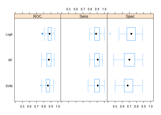
It can be concluded that all three models better predict the dead than the survivors (respectively, statistics Sensitivity and Specificity). But, in general, the statistical results of the models are not significantly different from each other. But, from the point of view of simplicity of the model and generalizing properties, I believe that the best results on a new unknown sample on average should be shown by logistic regression.
The next block of code applies the selected model to the estimated data and creates a file for uploading to the site.
After downloading the results of applying models to Kaggle, the SVM model showed the best results. Entering at the time of writing this work in the top 10% of the results, but, because before the end of the competition, the model is evaluated only in part of the data, then the final results can be very different, and both for the better and for the worse. Below are the results of evaluating models on Public data.
Thanks to everyone who was able to finish reading this post to the end!) I remind you that until November 30, you can still receive course materials on data analysis from the MLClass project
# {Data Science for newbies}
My name is Gleb Morozov, we are already familiar with the previous articles. Due to numerous requests, I continue to describe the experience of my participation in educational projects of MLClass.ru (by the way, who have not had time - you can still get the materials of past courses before the end - this is probably the shortest and most practical course in data analysis that you can imagine) .
This paper describes my attempt to create a model for predicting the surviving passengers of the Titanic. The main task is training in the use of tools used in Data Science for data analysis and presentation of research results, so this article will be very, very long . The focus is on exploratory research and on the creation and selection of predictors ( feature engineering ). The model is created as part of the Titanic: Machine Learning from Disaster competition on the Kaggle website. In my work I will use the language "R".
Prerequisites for creating a model
If you trust Wikipedia, then Titanic collided with an iceberg at 11:40 pm ship time, when the vast majority of passengers and ship crew were in their cabins. Accordingly, the location of the cabins may have had an impact on the likelihood of survival, since passengers of the lower decks, first, later learned about the collision and, accordingly, had less time to get to the upper deck. And, secondly, they naturally had to get out of the ship’s premises longer. Below are the schemes of the Titanic, indicating the decks and rooms.
')
The Titanic was a British ship, and according to the laws of Britain, the number of lifeboats that corresponded to the vessel’s displacement and not the passenger capacity had to be on the ship. Titanic formally met these requirements and had 20 boats (14 with a capacity of 65 people, 2 - 40 people, 4 - 47 people), which were designed to load 1178 people, just 2208 people on Titanic. Thus, knowing that there would not be enough boats for everyone, the captain of the Titanic Smith gave, after a collision with an iceberg, an order to take on boats only women and children. However, team members did not always follow him.
Data acquisition
Kaggle provides data as two files in csv format:
- train.csv (contains a sample of passengers with a known outcome, i.e. survived or not)
- test.csv (contains another sample of passengers without a dependent variable)
To get the data in R, I use the read_csv function from the readr package. In comparison with the basic functions, this package provides a number of advantages, in particular: higher speed and clear names of parameters.
require(readr) data_train <- read_csv("train.csv") data_test <- read_csv("test.csv") Let's see what we got:
str(data_train) ## Classes 'tbl_df', 'tbl' and 'data.frame': 891 obs. of 12 variables: ## $ PassengerId: int 1 2 3 4 5 6 7 8 9 10 ... ## $ Survived : int 0 1 1 1 0 0 0 0 1 1 ... ## $ Pclass : int 3 1 3 1 3 3 1 3 3 2 ... ## $ Name : chr "Braund, Mr. Owen Harris" "Cumings, Mrs. John Bradley (Florence Briggs Thayer)" "Heikkinen, Miss. Laina" "Futrelle, Mrs. Jacques Heath (Lily May Peel)" ... ## $ Sex : chr "male" "female" "female" "female" ... ## $ Age : num 22 38 26 35 35 NA 54 2 27 14 ... ## $ SibSp : int 1 1 0 1 0 0 0 3 0 1 ... ## $ Parch : int 0 0 0 0 0 0 0 1 2 0 ... ## $ Ticket : chr "A/5 21171" "PC 17599" "STON/O2. 3101282" "113803" ... ## $ Fare : num 7.25 71.28 7.92 53.1 8.05 ... ## $ Cabin : chr "" "C85" "" "C123" ... ## $ Embarked : chr "S" "C" "S" "S" ... Data analysis
I believe that research data analysis is one of the most important parts of Data Scientist's work, because, apart from directly transforming “raw” data into ready-made models, often during this process you can see hidden dependencies, thanks to which the most accurate models are obtained.
First, look at the missing data. In the data provided, a part of the missing information was marked with the symbol NA and, when loaded, were converted to the special symbol NA by default. But among symbolic variables there are many passengers with missing variables that were not marked. Check their availability using the capabilities of the packages magrittr and dplyr
require(magrittr) require(dplyr) data_train %>% select(Name, Sex, Ticket, Cabin, Embarked) %>% apply(., 2, function(column) sum(column == "")) ## Name Sex Ticket Cabin Embarked ## 0 0 0 687 2 Replace the blanks with NA, using the recode function from the car package.
require(car) data_train$Cabin <- recode(data_train$Cabin, "'' = NA") data_train$Embarked <- recode(data_train$Embarked, "'' = NA") For a graphical representation, it is convenient to use the missmap function from the package for working with missing Amelia data.
require(colorspace) colors_A <- sequential_hcl(2) require(Amelia) missmap(data_train, col = colors_A, legend=FALSE) Thus, about 20% of the data in the Age variable and almost 80% in Cabin are missing. And if with the age of the passengers it is possible to make a reasonable replacement of the missing values, due to their small share, then it is unlikely to do something with the cabins, because Missing values are significantly more than filled. Missing Values in the Embarked Tag
We will return to the missing values later, but for now let's see what information can be extracted from the data that we have. I remind you that the main task is to determine the variables that affect the probability of surviving a Titanic crash. Let's try to get initial ideas about these dependencies using simple graphs.
## 'ggplot2' require(ggplot2) require(gridExtra) data_train %<>% transform(., Survived = as.factor(Survived), Pclass = as.factor(Pclass), Sex = as.factor(Sex), Embarked = as.factor(Embarked), SibSp = as.numeric(SibSp)) colours <- rainbow_hcl(4, start = 30, end = 300) ggbar <- ggplot(data_train) + geom_bar(stat = "bin", width=.6, fill= colours[3], colour="black") + guides(fill=FALSE) + ylab(NULL) g1 <- ggbar + aes(x = factor(Survived, labels = c("", ""))) + ggtitle(" \n ") + xlab(NULL) g2 <- ggbar + aes(x = factor(Pclass, labels = c("", "", ""))) + ggtitle(" \n ") + xlab(NULL) g3 <- ggbar + aes(x = factor(Sex, labels = c("", ""))) + ggtitle(" ") + xlab(NULL) g4 <- ggbar + aes(x = as.factor(SibSp)) + ggtitle(" \n ' + '") + xlab(NULL) g5 <- ggbar + aes(x = as.factor(Parch)) + ggtitle(" \n ' + '") + xlab(NULL) g6 <- ggbar + aes(x = factor(Embarked, labels = c("Cherbourg", "Queenstown", "Southampton"))) + ggtitle(" \n ") + xlab(NULL) gghist <- ggplot(data_train) + geom_histogram(fill= colours[4]) + guides(fill=FALSE) + ylab(NULL) g7 <- gghist + aes(x = Age) + xlab(NULL) + ggtitle(" ") g8 <- gghist + aes(x = Fare) + xlab(NULL) + ggtitle(" \n ") grid.arrange(g1, g2, g3, g4, g5, g6, g7, g8, ncol = 2, nrow=4) Already it is possible to draw the first conclusions:
- more passengers were killed than saved
- the vast majority of passengers were in cabins of the third class
- there were more men than women
In general, we can already say that the main factors of the model will be the floor of the passenger (remember the order of the captain, about which I wrote earlier) and the location of the cabin.
Let's go back to the missing values for a while. From the schedule Distribution of passengers at the point of departure it is obvious that most of the passengers went from Southampton, respectively, you can safely replace 2 NA with this value
data_train$Embarked[is.na(data_train$Embarked)] <- "S" Now take a closer look at the relationship between the probability of survival and other factors. The following graph confirms the theory that the higher the passenger cabin class, the greater the chances of survival. (By "higher", "I mean the reverse order, because the first class is higher than the second and, especially, the third.)
ggbar <- ggplot(data_train) + geom_bar(stat = "bin", width=.6) ggbar + aes(x = factor(Pclass, labels = c("", "", "")), fill = factor(Survived, labels = c("", ""))) + scale_fill_manual (values=colours[]) + guides(fill=guide_legend(title=NULL)) + ylab(NULL) + xlab(" ") Compare the chances of survival in men and women. The data confirm the theory expressed earlier.
ggbar + aes(x = factor(Sex, labels = c("", "")), fill = factor(Survived, labels = c("", ""))) + scale_fill_manual (values=colours[]) + guides(fill=guide_legend(title=NULL)) + ylab(NULL) + xlab(" ") Now let's take a look at the chances of surviving passengers from various ports of departure.
ggbar + aes(x = factor(Embarked, labels = c("Cherbourg", "Queenstown", "Southampton")), fill = factor(Survived, labels = c("", ""))) + scale_fill_manual (values=colours[]) + guides(fill=guide_legend(title=NULL)) + ylab(NULL) + xlab(" ") It seems that there is some kind of connection, but I think that this is most likely due to the distribution of passengers of different classes between these ports, which is confirmed by the following graph.
ggbar + aes(x = factor(Embarked, labels = c("Cherbourg", "Queenstown", "Southampton")), fill = factor(Pclass, labels = c("", "", ""))) + scale_fill_manual (values=colours[]) + guides(fill=guide_legend(title=" ")) + ylab(NULL) + xlab(" ") You can also test the hypothesis that younger people survive, because they move faster, swim better, etc.
ggplot(data_train, aes(x = factor(Survived, labels = c("", "")), y = Age, fill = factor(Survived, labels = c("", "")))) + geom_boxplot() + scale_fill_manual (values=colours[]) + guides(fill=guide_legend(title=NULL)) + ylab(NULL) + xlab(NULL) As you can see, an obvious dependency is not visible here.
Now, with the help of another type of graph, let's look at the presence of possible statistical relationships between the features of objects. You can make preliminary conclusions that confirm the thoughts expressed earlier. In particular, that the chances of survival decrease with the growth of the class and age is a very weak symptom for building a model. You can also find other patterns. There is a negative correlation between age and class, which is most likely due to more aged passengers more often could afford a more expensive cabin. In addition, the ticket price and class are closely related (high correlation coefficient), which is quite expected.
source('my.plotcorr.R') corplot_data <- data_train %>% select(Survived, Pclass, Sex, Age, SibSp, Parch, Fare, Embarked) %>% mutate(Survived = as.numeric(Survived), Pclass = as.numeric(Pclass), Sex = as.numeric(Sex), Embarked = as.numeric(Embarked)) corr_train_data <- cor(corplot_data, use = "na.or.complete") colsc <- c(rgb(241, 54, 23, maxColorValue=255), 'white', rgb(0, 61, 104, maxColorValue=255)) colramp <- colorRampPalette(colsc, space='Lab') colorscor <- colramp(100) my.plotcorr(corr_train_data, col=colorscor[((corr_train_data + 1)/2) * 100], upper.panel="number", mar=c(1,2,1,1), main=' ') Let's go back to the missing values in the data. One of the usual ways to deal with them is to replace them with an average of the available values of the same trait. For example, 177 missed from the sign Age can be replaced by 29.7
summary(data_train$Age) ## Min. 1st Qu. Median Mean 3rd Qu. Max. NA's ## 0.42 20.12 28.00 29.70 38.00 80.00 177 I have already successfully applied this method earlier with the Embarked sign, but there were only two replacements, and here - 177, which is more than 20% of all available data on this sign. Therefore, it is worth finding a more accurate way to replace.
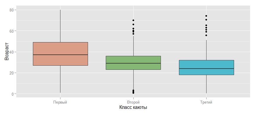
One of the possible options is to take the average, but depending on the class of the cabin, because if you look at the chart below, this relationship is possible. And, if you think about it, such an assumption is intuitively clear: the older a person is, the higher his probable well-being and, accordingly, the higher level of comfort that he can afford. Thus, it is possible to replace the missing value for a passenger, for example, from the third class, with the average age for this class, which will already be a great progress compared to just the average for all passengers.
ggplot(data_train, aes(x = factor(Pclass, labels = c("", "", "")), y = Age, fill = factor(Pclass))) + geom_boxplot() + scale_fill_manual (values=colours) + ylab("") + xlab(" ") + guides(fill=FALSE) But let's turn to another of the possible options for replacing the missing values for the Age attribute. If you look at the values of the Name attribute, you can notice an interesting feature.
head(data_train$Name) ## [1] "Braund, Mr. Owen Harris" ## [2] "Cumings, Mrs. John Bradley (Florence Briggs Thayer)" ## [3] "Heikkinen, Miss. Laina" ## [4] "Futrelle, Mrs. Jacques Heath (Lily May Peel)" ## [5] "Allen, Mr. William Henry" ## [6] "Moran, Mr. James" The name of each passenger is built one pattern each time: “Last Name, Gonorato. Name". The appeal of the Master in the 19th century was applied to male children, respectively, this can be used to single out narrower and more precise groups by age. And Miss was applied to unmarried women, but in the 19th century, in the overwhelming majority, only young girls and girls were unmarried. In order to use this dependency we will create a new Title attribute.
require(stringr) data_train$Title <- data_train$Name %>% str_extract(., "\\w+\\.") %>% str_sub(.,1, -2) unique(data_train$Title) ## [1] "Mr" "Mrs" "Miss" "Master" "Don" "Rev" ## [7] "Dr" "Mme" "Ms" "Major" "Lady" "Sir" ## [13] "Mlle" "Col" "Capt" "Countess" "Jonkheer" Now we define titles, among owners of which there is at least one with absent age.
mean_title <- data_train %>% group_by(Title) %>% summarise(count = n(), Missing = sum(is.na(Age)), Mean = round(mean(Age, na.rm = T), 2)) mean_title ## Source: local data frame [17 x 4] ## ## Title count Missing Mean ## 1 Capt 1 0 70.00 ## 2 Col 2 0 58.00 ## 3 Countess 1 0 33.00 ## 4 Don 1 0 40.00 ## 5 Dr 7 1 42.00 ## 6 Jonkheer 1 0 38.00 ## 7 Lady 1 0 48.00 ## 8 Major 2 0 48.50 ## 9 Master 40 4 4.57 ## 10 Miss 182 36 21.77 ## 11 Mlle 2 0 24.00 ## 12 Mme 1 0 24.00 ## 13 Mr 517 119 32.37 ## 14 Mrs 125 17 35.90 ## 15 Ms 1 0 28.00 ## 16 Rev 6 0 43.17 ## 17 Sir 1 0 49.00 And we will replace. To do this, create a function and apply it to the attribute Age.
impute.mean <- function (impute_col, filter_var, var_levels) { for (lev in var_levels) { impute_col[(filter_var == lev) & is.na(impute_col)] <- mean(impute_col[filter_var == lev], na.rm = T) } return (impute_col) } data_train$Age <- impute.mean(data_train$Age, data_train$Title, c("Dr", "Master", "Mrs", "Miss", "Mr")) summary(data_train$Age) ## Min. 1st Qu. Median Mean 3rd Qu. Max. ## 0.42 21.77 30.00 29.75 35.90 80.00 If you pay attention to the sign of Fare (ticket price), you can see that there are tickets with zero cost.
head(table(data_train$Fare)) ## ## 0 4.0125 5 6.2375 6.4375 6.45 ## 15 1 1 1 1 1 The first explanation that comes to mind is the children, but if you look at the other signs of these passengers, this assumption turns out to be false.
data_train %>% filter(Fare < 6) %>% select(Fare, Age, Pclass, Title) %>% arrange(Fare) ## Fare Age Pclass Title ## 1 0.0000 36.00000 3 Mr ## 2 0.0000 40.00000 1 Mr ## 3 0.0000 25.00000 3 Mr ## 4 0.0000 32.36809 2 Mr ## 5 0.0000 19.00000 3 Mr ## 6 0.0000 32.36809 2 Mr ## 7 0.0000 32.36809 2 Mr ## 8 0.0000 32.36809 2 Mr ## 9 0.0000 49.00000 3 Mr ## 10 0.0000 32.36809 1 Mr ## 11 0.0000 32.36809 2 Mr ## 12 0.0000 32.36809 2 Mr ## 13 0.0000 39.00000 1 Mr ## 14 0.0000 32.36809 1 Mr ## 15 0.0000 38.00000 1 Jonkheer ## 16 4.0125 20.00000 3 Mr ## 17 5.0000 33.00000 1 Mr Therefore, I think it would be logical to replace the zero values with the average values for the class using the already used impute.mean function.
data_train$Fare[data_train$Fare == 0] <- NA data_train$Fare <- impute.mean(data_train$Fare, data_train$Pclass, as.numeric(levels(data_train$Pclass))) The Title attribute, introduced to replace missing values in the Age attribute, gives us additional information about the passenger field, its nobility (for example, Don and Sir) and the priority in accessing the lifeboats. Therefore, this feature must be left when building a model. In total, we have 17 values of this attribute. The following graph shows their relationship with age.
ggplot(data_train, aes(x = factor(Title, c("Capt","Col","Major","Sir","Lady","Rev", "Dr","Don","Jonkheer","Countess","Mrs", "Ms","Mr","Mme","Mlle","Miss","Master")), y = Age)) + geom_boxplot(fill= colours[3]) + guides(fill=FALSE) + guides(fill=guide_legend(title=NULL)) + ylab("") + xlab(NULL) But many of the values, as I believe, can be combined into 5 groups: Aristocratic, Mr, Mrs, Miss and Master, since merged titles belong in fact to one or related groups.
change.titles <- function(data, old_title, new_title) { for (title in old_title) { data$Title[data$Title == title] <- new_title } return (data$Title) } data_train$Title <- change.titles(data_train, c("Capt", "Col", "Don", "Dr", "Jonkheer", "Lady", "Major", "Rev", "Sir", "Countess"), "Aristocratic") data_train$Title <- change.titles(data_train, c("Ms"), "Mrs") data_train$Title <- change.titles(data_train, c("Mlle", "Mme"), "Miss") data_train$Title <- as.factor(data_train$Title) ggplot(data_train, aes(x = factor(Title, c("Aristocratic", "Mrs", "Mr", "Miss", "Master")), y = Age)) + geom_boxplot(fill= colours[3]) + guides(fill=FALSE) + guides(fill=guide_legend(title=NULL)) + ylab("") + xlab(NULL) Let's introduce such an indicator as Survival Percentage and look at its dependence on the groups that turned out at the previous stage.
Surv_rate_title <- data_train %>% group_by(Title) %>% summarise(Rate = mean(as.numeric(as.character(Survived)))) ggplot(Surv_rate_title, aes(x = Title, y = Rate)) + geom_bar(stat = "identity", width=.6, fill= colours[3]) + xlab(NULL) + ylab(" ") In order to get a good idea of the relationship between the signs is better than the graphics, as I think nothing has yet been invented. For example, according to the following graph, it is clearly seen that the main groups of survivors are women of the first and second class of all ages. And among the men, all the boys younger than 15 years old survived except the third class of service and a small proportion of older men and mostly from the first class.
ggplot(data = data_train, aes(x = Age, y = Pclass, color = factor(Survived, labels = c("", "")))) + geom_point(shape = 1, size = 4, position=position_jitter(width=0.1,height=.1)) + facet_grid(Sex ~ .) + guides(color=guide_legend(title=NULL)) + xlab("") + ylab(" ") Now look at the information that can be obtained from the number of relatives on the ship.
ggplot(data_train, aes(x = SibSp, y = Parch, color = factor(Survived, labels = c("", "")))) + geom_point(shape = 1, size = 4, position=position_jitter(width=0.3,height=.3)) + guides(color=guide_legend(title=NULL)) + xlab("- \n ,\n .. , ") + ylab("- \n ,\n .. , ..") It is very likely that survival is negatively affected by the absence of relatives as well as a large number.
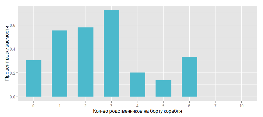
We introduce such a feature as Family, i.e. the number of relatives on board the ship and look at the effect on survival.
Surv_rate_family <- data_train %>% group_by(Family = SibSp + Parch) %>% summarise(Rate = mean(as.numeric(as.character(Survived)))) ggplot(Surv_rate_family, aes(x = as.factor(Family), y = Rate)) + geom_bar(stat = "identity", width=.6, fill= colours[3]) + xlab("- ") + ylab(" ") And also in the context of the sexes of passengers.
data_train$Family <- data_train$SibSp + data_train$Parch ggplot(data_train, aes(x = factor(Family), y = as.numeric(as.character(Survived)))) + stat_summary( fun.y = mean, ymin=0, ymax=1, geom="bar", size=4, fill= colours[2]) + xlab("- ") + ylab(" ") + facet_grid(Sex ~ .) The graph shows that for a woman a small number of relatives significantly increases the likelihood of survival. The statistical significance of this dependence should be checked, but I think that the attribute should be left and to look at its influence when creating the model. It is also possible that such a binary sign as “Having relatives on board” will make sense.
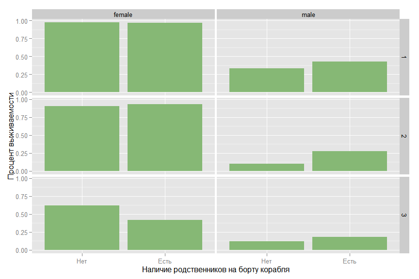
data_train$isFamily <- as.factor(as.numeric(data_train$Family > 0)) ggplot( data_train, aes(x=factor(isFamily, labels =c("", "")),y=as.numeric(as.character(Survived))) ) + stat_summary( fun.y = mean, ymin=0, ymax=1, geom="bar", size=4, fill= colours[2]) + ylab(" ") + xlab(" ") At first glance, it seems that the presence of relatives increases the likelihood of survival, but if you look at the relationship in terms of classes and gender, the picture changes.
ggplot(data_train, aes(x = factor(isFamily, labels =c("", "")), y = as.numeric(as.character(Survived)))) + stat_summary( fun.y = "mean", geom="bar", ymin=0, ymax=1, fill= colours[2]) + facet_grid(Pclass ~ Sex) + ylab(" ") + xlab(" ") For a man in the second grade, relatives increase survival, but for a woman in the third grade, the situation is reversed.
From the sign of Cabin, i.e. cabin numbers occupied by the passenger, it would be possible to extract the deck number (this is the letter in the room) and on which board the cabin was (if the last digit of the number is odd, then this is the port side, and, accordingly, vice versa), but since only 20% of passengers have cabin numbers in the data, I do not think that this will significantly affect the accuracy of the model. Much more interesting, in my opinion, will be information about the availability of this number. The first-class cabin numbers became known from the list that was found on the body of the steward Herbert Cave, no further official information was preserved, respectively, it can be concluded that if the passenger room number of the second or third class is known, then he survived. Therefore, as with relatives, we will look at survival depending on the availability of a cabin room as a whole for all passengers and in a section by class and sex.
data_train$isCabin <- factor(ifelse(is.na(data_train$Cabin),0,1)) ggplot( data_train, aes(x=factor(isCabin, labels =c("", "")),y=as.numeric(as.character(Survived))) ) + stat_summary( fun.y = mean, ymin=0, ymax=1, geom="bar", size=4, fill= colours[3]) + ylab(" ") + xlab(" ") ggplot(data_train, aes(x = factor(isCabin, labels =c("", "")), y = as.numeric(as.character(Survived)))) + stat_summary( fun.y = "mean", geom="bar", ymin=0, ymax=1, fill= colours[3]) + facet_grid(Pclass ~ Sex) + ylab(" ") + xlab(" ") Obviously, the assumption was confirmed, especially for male passengers.
To summarize all the research work that has been done:
- Certain patterns were identified in the data, but in order to say for sure that the target attribute depends on this and on this it is necessary to conduct a statistical analysis.
- Additional features were created Title, Family, isFamily, isCabin, which, in my opinion, have an impact on the target feature and can be used to create the model. But the final conclusion about the benefits of these features can be made only in the process of creating a predictive model.
Now select from the data those signs that we will use when creating the model.
data_train %<>% select(Survived, Pclass, Sex, Age, Fare, Embarked, Title, Family, isFamily, isCabin) And the last schedule in this part of the work.
corplot_data <- data_train %>% select(Survived, Pclass, Sex, Age, Fare, Embarked, Family, isFamily, isCabin) %>% mutate(Survived = as.numeric(Survived), Pclass = as.numeric(Pclass), Sex = as.numeric(Sex), Embarked = as.numeric(Embarked), isFamily = as.numeric(isFamily), isCabin = as.numeric(isCabin)) corr_train_data <- cor(corplot_data, use = "na.or.complete") colsc <- c(rgb(241, 54, 23, maxColorValue=255), 'white', rgb(0, 61, 104, maxColorValue=255)) colramp <- colorRampPalette(colsc, space='Lab') colorscor <- colramp(100) my.plotcorr(corr_train_data, col=colorscor[((corr_train_data + 1)/2) * 100], upper.panel="number", mar=c(1,2,1,1), main=' ') Prepare data for correct use in the process models.
require(plyr) require(dplyr) data_train$Survived %<>% revalue(., c("0"="Died", "1" = "Survived")) data_train$Pclass %<>% revalue(., c("1"="First", "2"="Second", "3"="Third")) data_train$Sex %<>% revalue(., c("female"="Female", "male"="Male")) data_train$isFamily %<>% revalue(., c("0"="No", "1"="Yes")) data_train$isCabin %<>% revalue(., c("0"="No", "1"="Yes")) Creating a model
In this paper, I will use the caret package, which has absorbed most of the well-known models of machine learning and provides a convenient interface for their practical use. Despite the fact that we have a test sample provided by the Kaggle site, we still need to split the training sample into two parts. On one of which we will train the model, and on the other, we will evaluate its quality before applying it to a competitive sample. I chose an 80/20 split.
require(caret) set.seed(111) split <- createDataPartition(data_train$Survived, p = 0.8, list = FALSE) train <- slice(data_train, split) test <- slice(data_train, -split) Let's start with the simplest classification model - logistic regression. To evaluate the model, we will use the residual deviance statistics or residual deviation, which indirectly corresponds to the variance in the data, which is unexplained after the model has been applied. Null deviance or null deviance is the deviation of the “empty” model, which does not include any parameters other than beta0. Accordingly, the smaller the deviation of residuals in relation to the null deviance - the better the model. In the future, to compare different models, AUC statistics or the area under the ROC curve will be used.To correctly estimate this parameter, it will be estimated using a tenfold cross-validation (10-fold cross-validation (CV)) with the sample split into 10 parts.
So the first model is logistic regression. Predictors initially present in the data provided are selected as features.
cv_ctrl <- trainControl(method = "repeatedcv", repeats = 10, summaryFunction = twoClassSummary, classProbs = TRUE) set.seed(111) glm.tune.1 <- train(Survived ~ Pclass + Sex + Age + Fare + Embarked + Family, data = train, method = "glm", metric = "ROC", trControl = cv_ctrl) glm.tune.1 ## Generalized Linear Model ## ## 714 samples ## 9 predictor ## 2 classes: 'Died', 'Survived' ## ## No pre-processing ## Resampling: Cross-Validated (10 fold, repeated 10 times) ## Summary of sample sizes: 643, 643, 643, 642, 643, 642, ... ## Resampling results ## ## ROC Sens Spec ROC SD Sens SD Spec SD ## 0.8607813 0.8509091 0.7037963 0.0379468 0.05211929 0.08238326 ## ## summary(glm.tune.1) ## ## Call: ## NULL ## ## Deviance Residuals: ## Min 1Q Median 3Q Max ## -2.2611 -0.5641 -0.3831 0.5944 2.5244 ## ## Coefficients: ## Estimate Std. Error z value Pr(>|z|) ## (Intercept) 4.5920291 0.5510121 8.334 < 2e-16 *** ## PclassSecond -1.0846865 0.3449892 -3.144 0.00167 ** ## PclassThird -2.5390919 0.3469115 -7.319 2.50e-13 *** ## SexMale -2.7351467 0.2277348 -12.010 < 2e-16 *** ## Age -0.0450577 0.0088554 -5.088 3.62e-07 *** ## Fare 0.0002526 0.0028934 0.087 0.93042 ## EmbarkedQ -0.1806726 0.4285553 -0.422 0.67333 ## EmbarkedS -0.4364064 0.2711112 -1.610 0.10746 ## Family -0.1973088 0.0805129 -2.451 0.01426 * ## --- ## Signif. codes: 0 '***' 0.001 '**' 0.01 '*' 0.05 '.' 0.1 ' ' 1 ## ## (Dispersion parameter for binomial family taken to be 1) ## ## Null deviance: 950.86 on 713 degrees of freedom ## Residual deviance: 613.96 on 705 degrees of freedom ## AIC: 631.96 ## ## Number of Fisher Scoring iterations: 5 The model already shows good performance in reducing deviance by 950-613 = 337 points compared to the “empty” model. Now we will try to improve this indicator by entering those new features that were added earlier.
set.seed(111) glm.tune.2 <- train(Survived ~ Pclass + Sex + Age + Fare + Embarked + Title + Family + isFamily + isCabin, data = train, method = "glm", metric = "ROC", trControl = cv_ctrl) glm.tune.2 ## Generalized Linear Model ## ## 714 samples ## 9 predictor ## 2 classes: 'Died', 'Survived' ## ## No pre-processing ## Resampling: Cross-Validated (10 fold, repeated 10 times) ## Summary of sample sizes: 643, 643, 643, 642, 643, 642, ... ## Resampling results ## ## ROC Sens Spec ROC SD Sens SD Spec SD ## 0.8755115 0.8693182 0.7661772 0.03599347 0.04526764 0.07882857 ## ## summary(glm.tune.2) ## ## Call: ## NULL ## ## Deviance Residuals: ## Min 1Q Median 3Q Max ## -2.4368 -0.5285 -0.3532 0.5087 2.5409 ## ## Coefficients: ## Estimate Std. Error z value Pr(>|z|) ## (Intercept) 1.467e+01 5.354e+02 0.027 0.978145 ## PclassSecond -4.626e-01 4.765e-01 -0.971 0.331618 ## PclassThird -1.784e+00 4.790e-01 -3.725 0.000195 *** ## SexMale -1.429e+01 5.354e+02 -0.027 0.978701 ## Age -3.519e-02 1.093e-02 -3.221 0.001279 ** ## Fare 2.175e-04 2.828e-03 0.077 0.938704 ## EmbarkedQ -1.405e-01 4.397e-01 -0.320 0.749313 ## EmbarkedS -4.426e-01 2.887e-01 -1.533 0.125224 ## TitleMaster 3.278e+00 8.805e-01 3.722 0.000197 *** ## TitleMiss -1.120e+01 5.354e+02 -0.021 0.983313 ## TitleMr 2.480e-01 6.356e-01 0.390 0.696350 ## TitleMrs -1.029e+01 5.354e+02 -0.019 0.984660 ## Family -4.841e-01 1.240e-01 -3.903 9.49e-05 *** ## isFamilyYes 2.248e-01 3.513e-01 0.640 0.522266 ## isCabinYes 1.060e+00 4.122e-01 2.572 0.010109 * ## --- ## Signif. codes: 0 '***' 0.001 '**' 0.01 '*' 0.05 '.' 0.1 ' ' 1 ## ## (Dispersion parameter for binomial family taken to be 1) ## ## Null deviance: 950.86 on 713 degrees of freedom ## Residual deviance: 566.46 on 699 degrees of freedom ## AIC: 596.46 ## ## Number of Fisher Scoring iterations: 12 <source> ! 613-566=47 . , , , -, Sex, , .. Title . Fare, .. . Embarked, . <source code="R"> set.seed(111) glm.tune.3 <- train(Survived ~ Pclass + Age + I(Embarked=="S") + Title + Family + isFamily + isCabin, data = train, method = "glm", metric = "ROC", trControl = cv_ctrl) glm.tune.3 ## Generalized Linear Model ## ## 714 samples ## 9 predictor ## 2 classes: 'Died', 'Survived' ## ## No pre-processing ## Resampling: Cross-Validated (10 fold, repeated 10 times) ## Summary of sample sizes: 643, 643, 643, 642, 643, 642, ... ## Resampling results ## ## ROC Sens Spec ROC SD Sens SD Spec SD ## 0.8780578 0.8702273 0.7705423 0.03553343 0.04502726 0.07757737 ## ## summary(glm.tune.3) ## ## Call: ## NULL ## ## Deviance Residuals: ## Min 1Q Median 3Q Max ## -2.4508 -0.5286 -0.3522 0.5120 2.5449 ## ## Coefficients: ## Estimate Std. Error z value Pr(>|z|) ## (Intercept) 0.55401 0.80063 0.692 0.48896 ## PclassSecond -0.49217 0.44618 -1.103 0.26999 ## PclassThird -1.81552 0.42912 -4.231 2.33e-05 *** ## Age -0.03554 0.01083 -3.281 0.00103 ** ## `I(Embarked == "S")TRUE` -0.37801 0.24222 -1.561 0.11862 ## TitleMaster 3.06205 0.84703 3.615 0.00030 *** ## TitleMiss 2.88073 0.64386 4.474 7.67e-06 *** ## TitleMr 0.04083 0.58762 0.069 0.94460 ## TitleMrs 3.80377 0.67946 5.598 2.17e-08 *** ## Family -0.48442 0.12274 -3.947 7.93e-05 *** ## isFamilyYes 0.22652 0.34724 0.652 0.51418 ## isCabinYes 1.08796 0.40990 2.654 0.00795 ** ## --- ## Signif. codes: 0 '***' 0.001 '**' 0.01 '*' 0.05 '.' 0.1 ' ' 1 ## ## (Dispersion parameter for binomial family taken to be 1) ## ## Null deviance: 950.86 on 713 degrees of freedom ## Residual deviance: 568.64 on 702 degrees of freedom ## AIC: 592.64 ## ## Number of Fisher Scoring iterations: 5 , , , . , ROC, , p-value , , , . . isFamily, .. Family . , . Title.
set.seed(111) glm.tune.4 <- train(Survived ~ I(Pclass=="Third") + Age + I(Embarked=="S") + I(Title=="Master") + I(Title=="Miss") + I(Title=="Mrs") + Family + isCabin, data = train, method = "glm", metric = "ROC", trControl = cv_ctrl) glm.tune.4 ## Generalized Linear Model ## ## 714 samples ## 9 predictor ## 2 classes: 'Died', 'Survived' ## ## No pre-processing ## Resampling: Cross-Validated (10 fold, repeated 10 times) ## Summary of sample sizes: 643, 643, 643, 642, 643, 642, ... ## Resampling results ## ## ROC Sens Spec ROC SD Sens SD Spec SD ## 0.8797817 0.8738636 0.7719841 0.03535413 0.04374363 0.0775346 ## ## summary(glm.tune.4) ## ## Call: ## NULL ## ## Deviance Residuals: ## Min 1Q Median 3Q Max ## -2.4369 -0.5471 -0.3533 0.5098 2.5384 ## ## Coefficients: ## Estimate Std. Error z value Pr(>|z|) ## (Intercept) 0.29594 0.46085 0.642 0.520765 ## `I(Pclass == "Third")TRUE` -1.46194 0.26518 -5.513 3.53e-08 *** ## Age -0.03469 0.01049 -3.306 0.000946 *** ## `I(Embarked == "S")TRUE` -0.45389 0.23350 -1.944 0.051910 . ## `I(Title == "Master")TRUE` 3.01939 0.59974 5.035 4.79e-07 *** ## `I(Title == "Miss")TRUE` 2.83185 0.29232 9.687 < 2e-16 *** ## `I(Title == "Mrs")TRUE` 3.80006 0.36823 10.320 < 2e-16 *** ## Family -0.42962 0.09269 -4.635 3.57e-06 *** ## isCabinYes 1.43072 0.30402 4.706 2.53e-06 *** ## --- ## Signif. codes: 0 '***' 0.001 '**' 0.01 '*' 0.05 '.' 0.1 ' ' 1 ## ## (Dispersion parameter for binomial family taken to be 1) ## ## Null deviance: 950.86 on 713 degrees of freedom ## Residual deviance: 570.25 on 705 degrees of freedom ## AIC: 588.25 ## ## Number of Fisher Scoring iterations: 5 , .., , .
set.seed(111) glm.tune.5 <- train(Survived ~ Pclass + Age + I(Embarked=="S") + I(Title=="Master") + I(Title=="Miss") + I(Title=="Mrs") + Family + isCabin + I(Title=="Mr"& Pclass=="Third"), data = train, method = "glm", metric = "ROC", trControl = cv_ctrl) glm.tune.5 ## Generalized Linear Model ## ## 714 samples ## 9 predictor ## 2 classes: 'Died', 'Survived' ## ## No pre-processing ## Resampling: Cross-Validated (10 fold, repeated 10 times) ## Summary of sample sizes: 643, 643, 643, 642, 643, 642, ... ## Resampling results ## ## ROC Sens Spec ROC SD Sens SD Spec SD ## 0.8814059 0.8981818 0.7201455 0.03712511 0.04155444 0.08581645 ## ## summary(glm.tune.5) ## ## Call: ## NULL ## ## Deviance Residuals: ## Min 1Q Median 3Q Max ## -2.9364 -0.5340 -0.4037 0.3271 2.5123 ## ## Coefficients: ## Estimate Std. Error z value ## (Intercept) 0.52451 0.60337 0.869 ## PclassSecond -0.95649 0.52602 -1.818 ## PclassThird -3.54288 0.66944 -5.292 ## Age -0.03581 0.01126 -3.179 ## `I(Embarked == "S")TRUE` -0.46028 0.23707 -1.942 ## `I(Title == "Master")TRUE` 4.72492 0.80338 5.881 ## `I(Title == "Miss")TRUE` 4.43875 0.56446 7.864 ## `I(Title == "Mrs")TRUE` 5.24324 0.58650 8.940 ## Family -0.41607 0.09926 -4.192 ## isCabinYes 1.12486 0.42860 2.625 ## `I(Title == "Mr" & Pclass == "Third")TRUE` 2.30163 0.59547 3.865 ## Pr(>|z|) ## (Intercept) 0.384683 ## PclassSecond 0.069012 . ## PclassThird 1.21e-07 *** ## Age 0.001477 ** ## `I(Embarked == "S")TRUE` 0.052195 . ## `I(Title == "Master")TRUE` 4.07e-09 *** ## `I(Title == "Miss")TRUE` 3.73e-15 *** ## `I(Title == "Mrs")TRUE` < 2e-16 *** ## Family 2.77e-05 *** ## isCabinYes 0.008677 ** ## `I(Title == "Mr" & Pclass == "Third")TRUE` 0.000111 *** ## --- ## Signif. codes: 0 '***' 0.001 '**' 0.01 '*' 0.05 '.' 0.1 ' ' 1 ## ## (Dispersion parameter for binomial family taken to be 1) ## ## Null deviance: 950.86 on 713 degrees of freedom ## Residual deviance: 550.82 on 703 degrees of freedom ## AIC: 572.82 ## ## Number of Fisher Scoring iterations: 6 And we got a significant leap as a model. At this stage, we’ll stop with logistic regression and turn to other models.
In particular, to the very popular Random Forest. When training this model, you can choose the number of randomly selected, for each of the many trees created, signs - mtry.
rf.grid <- data.frame(.mtry = c(2, 3, 4)) set.seed(111) rf.tune <- train(Survived ~ Pclass + Sex + Age + Fare + Embarked + Title + Family + isFamily + isCabin, data = train, method = "rf", metric = "ROC", tuneGrid = rf.grid, trControl = cv_ctrl) rf.tune ## Random Forest ## ## 714 samples ## 9 predictor ## 2 classes: 'Died', 'Survived' ## ## No pre-processing ## Resampling: Cross-Validated (10 fold, repeated 10 times) ## Summary of sample sizes: 643, 643, 643, 642, 643, 642, ... ## Resampling results across tuning parameters: ## ## mtry ROC Sens Spec ROC SD Sens SD ## 2 0.8710121 0.8861364 0.7230423 0.03912907 0.04551133 ## 3 0.8723865 0.8929545 0.7021825 0.04049427 0.04467829 ## 4 0.8719942 0.8893182 0.7079630 0.04063512 0.04632489 ## Spec SD ## 0.08343852 ## 0.08960364 ## 0.08350602 ## ## ROC was used to select the optimal model using the largest value. ## The final value used for the model was mtry = 3. In this case, the best performance has a model with mtry equal to 3.
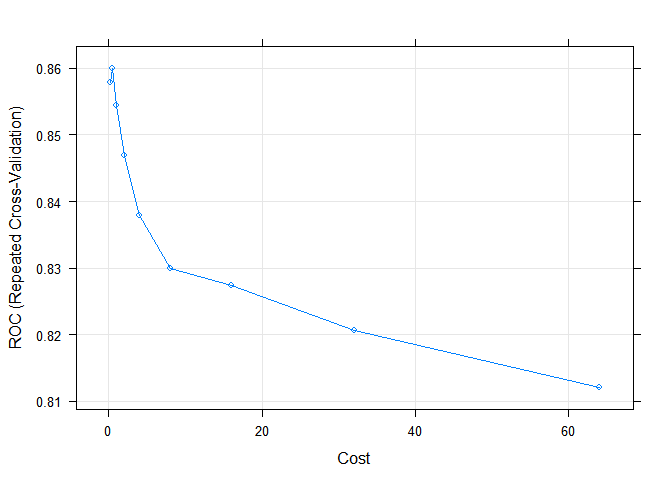
And the last model that will be used in this work is the support vector machine (SVM). SVM is sensitive to unnormalized input data, so the preProcess parameter will be used so that the model can be normalized before training the model. In SVM, Cost is used as one of the parameters. The model will be performed at its 9 different values and selected with the best AUC values.
set.seed(111) svm.tune <- train(Survived ~ Pclass + Sex + Age + Fare + Embarked + Title + Family + isFamily + isCabin, data = train, method = "svmRadial", tuneLength = 9, preProcess = c("center", "scale"), metric = "ROC", trControl = cv_ctrl) svm.tune ## Support Vector Machines with Radial Basis Function Kernel ## ## 714 samples ## 9 predictor ## 2 classes: 'Died', 'Survived' ## ## Pre-processing: centered, scaled ## Resampling: Cross-Validated (10 fold, repeated 10 times) ## Summary of sample sizes: 643, 643, 643, 642, 643, 642, ... ## Resampling results across tuning parameters: ## ## C ROC Sens Spec ROC SD Sens SD ## 0.25 0.8578892 0.8893182 0.7026455 0.04086454 0.04863259 ## 0.50 0.8599136 0.8956818 0.6862831 0.04005935 0.04952978 ## 1.00 0.8544741 0.8945455 0.6877646 0.04193910 0.04470456 ## 2.00 0.8469004 0.8943182 0.6814815 0.04342792 0.04595398 ## 4.00 0.8379595 0.8925000 0.6781746 0.04709993 0.04450981 ## 8.00 0.8299511 0.8877273 0.6769974 0.04692596 0.04403429 ## 16.00 0.8273934 0.8818182 0.6758862 0.04636108 0.04499307 ## 32.00 0.8206023 0.8756818 0.6769709 0.04665624 0.04339395 ## 64.00 0.8121454 0.8704545 0.6710714 0.04718058 0.04664421 ## Spec SD ## 0.08976378 ## 0.08597689 ## 0.08439794 ## 0.08532505 ## 0.08531935 ## 0.08434585 ## 0.07958467 ## 0.07687452 ## 0.07680478 ## ## Tuning parameter 'sigma' was held constant at a value of 0.1001103 ## ROC was used to select the optimal model using the largest value. ## The final values used for the model were sigma = 0.1001103 and C = 0.5. plot(svm.tune) Model evaluation
For all three models created, we will evaluate using the intersection of the predicted values and the real values of the target characteristic predicted on the test sample. Caret's confusionMatrix makes this easy to do.
glm.pred <- predict(glm.tune.4, test) confusionMatrix(glm.pred, test$Survived) ## Confusion Matrix and Statistics ## ## Reference ## Prediction Died Survived ## Died 92 15 ## Survived 17 53 ## ## Accuracy : 0.8192 ## 95% CI : (0.7545, 0.8729) ## No Information Rate : 0.6158 ## P-Value [Acc > NIR] : 3.784e-09 ## ## Kappa : 0.62 ## Mcnemar's Test P-Value : 0.8597 ## ## Sensitivity : 0.8440 ## Specificity : 0.7794 ## Pos Pred Value : 0.8598 ## Neg Pred Value : 0.7571 ## Prevalence : 0.6158 ## Detection Rate : 0.5198 ## Detection Prevalence : 0.6045 ## Balanced Accuracy : 0.8117 ## ## 'Positive' Class : Died ## rf.pred <- predict(rf.tune, test) confusionMatrix(rf.pred, test$Survived) ## Confusion Matrix and Statistics ## ## Reference ## Prediction Died Survived ## Died 103 18 ## Survived 6 50 ## ## Accuracy : 0.8644 ## 95% CI : (0.805, 0.9112) ## No Information Rate : 0.6158 ## P-Value [Acc > NIR] : 2.439e-13 ## ## Kappa : 0.7036 ## Mcnemar's Test P-Value : 0.02474 ## ## Sensitivity : 0.9450 ## Specificity : 0.7353 ## Pos Pred Value : 0.8512 ## Neg Pred Value : 0.8929 ## Prevalence : 0.6158 ## Detection Rate : 0.5819 ## Detection Prevalence : 0.6836 ## Balanced Accuracy : 0.8401 ## ## 'Positive' Class : Died ## svm.pred <- predict(svm.tune, test) confusionMatrix(svm.pred, test$Survived) ## Confusion Matrix and Statistics ## ## Reference ## Prediction Died Survived ## Died 101 17 ## Survived 8 51 ## ## Accuracy : 0.8588 ## 95% CI : (0.7986, 0.9065) ## No Information Rate : 0.6158 ## P-Value [Acc > NIR] : 9.459e-13 ## ## Kappa : 0.6939 ## Mcnemar's Test P-Value : 0.1096 ## ## Sensitivity : 0.9266 ## Specificity : 0.7500 ## Pos Pred Value : 0.8559 ## Neg Pred Value : 0.8644 ## Prevalence : 0.6158 ## Detection Rate : 0.5706 ## Detection Prevalence : 0.6667 ## Balanced Accuracy : 0.8383 ## ## 'Positive' Class : Died ## Random Forest shows the best result in predicting the dead - an indicator of Sensitivity. And logistic regression in predicting survivors is an indicator of Specificity.
Let's draw on the same graph the ROC curves on the test data for all the models created.
require(pROC) glm.probs <- predict(glm.tune.5, test, type = "prob") glm.ROC <- roc(response = test$Survived, predictor = glm.probs$Survived, levels = levels(test$Survived)) glm.ROC$auc ## Area under the curve: 0.8546 plot(glm.ROC, type="S") ## ## Call: ## roc.default(response = test$Survived, predictor = glm.probs$Survived, levels = levels(test$Survived)) ## ## Data: glm.probs$Survived in 109 controls (test$Survived Died) < 68 cases (test$Survived Survived). ## Area under the curve: 0.8546 rf.probs <- predict(rf.tune, test, type = "prob") rf.ROC <- roc(response = test$Survived, predictor = rf.probs$Survived, levels = levels(test$Survived)) rf.ROC$auc ## Area under the curve: 0.8854 plot(rf.ROC, add=TRUE, col="red") ## ## Call: ## roc.default(response = test$Survived, predictor = rf.probs$Survived, levels = levels(test$Survived)) ## ## Data: rf.probs$Survived in 109 controls (test$Survived Died) < 68 cases (test$Survived Survived). ## Area under the curve: 0.8854 svm.probs <- predict(svm.tune, test, type = "prob") svm.ROC <- roc(response = test$Survived, predictor = svm.probs$Survived, levels = levels(test$Survived)) svm.ROC$auc ## Area under the curve: 0.8714 plot(svm.ROC, add=TRUE, col="blue") ## ## Call: ## roc.default(response = test$Survived, predictor = svm.probs$Survived, levels = levels(test$Survived)) ## ## Data: svm.probs$Survived in 109 controls (test$Survived Died) < 68 cases (test$Survived Survived). ## Area under the curve: 0.8714 According to AUC statistics, Random Forest leads, but these are the results of a single application of the model on a test sample. If we collect these statistics by resampling, the result will be different, as shown in the following graph.
resamps <- resamples(list(Logit = glm.tune.5, RF = rf.tune, SVM = svm.tune)) summary(resamps) ## ## Call: ## summary.resamples(object = resamps) ## ## Models: Logit, RF, SVM ## Number of resamples: 100 ## ## ROC ## Min. 1st Qu. Median Mean 3rd Qu. Max. NA's ## Logit 0.7816 0.8608 0.8845 0.8814 0.9064 0.9558 0 ## RF 0.7715 0.8454 0.8732 0.8724 0.9048 0.9474 0 ## SVM 0.7593 0.8364 0.8620 0.8599 0.8845 0.9381 0 ## ## Sens ## Min. 1st Qu. Median Mean 3rd Qu. Max. NA's ## Logit 0.7955 0.8636 0.8864 0.8982 0.9318 1.0000 0 ## RF 0.7955 0.8636 0.9091 0.8930 0.9318 0.9773 0 ## SVM 0.7727 0.8636 0.9091 0.8957 0.9318 1.0000 0 ## ## Spec ## Min. 1st Qu. Median Mean 3rd Qu. Max. NA's ## Logit 0.4286 0.6667 0.7275 0.7201 0.7857 0.8889 0 ## RF 0.4815 0.6296 0.7037 0.7022 0.7778 0.8889 0 ## SVM 0.5000 0.6296 0.6786 0.6863 0.7500 0.8889 0 dotplot(resamps, metric = "ROC") And finally, the last schedule of this work. This is a summary of the models for the three statistics: ROC, Sensitivity and Specificity.
bwplot(resamps, layout = c(3, 1)) It can be concluded that all three models better predict the dead than the survivors (respectively, statistics Sensitivity and Specificity). But, in general, the statistical results of the models are not significantly different from each other. But, from the point of view of simplicity of the model and generalizing properties, I believe that the best results on a new unknown sample on average should be shown by logistic regression.
Using results for Kaggle
The next block of code applies the selected model to the estimated data and creates a file for uploading to the site.
data_test$Cabin <- recode(data_test$Cabin, "'' = NA") data_test$Embarked <- recode(data_test$Embarked, "'' = NA") data_test %<>% transform(.,Pclass = as.factor(Pclass), Sex = as.factor(Sex), Embarked = as.factor(Embarked), SibSp = as.numeric(SibSp)) data_test$Embarked[is.na(data_test$Embarked)] <- "S" data_test$Title <- data_test$Name %>% str_extract(., "\\w+\\.") %>% str_sub(.,1, -2) data_test %>% group_by(Title) %>% summarise(count = n(), Missing = sum(is.na(Age)), Mean = round(mean(Age, na.rm = T), 2)) impute.mean.test <- function (impute_col, filter_var, var_levels) { for (lev in var_levels) { impute_col[(filter_var == lev) & is.na(impute_col)] <- mean_title$Mean[mean_title$Title == lev] #mean(impute_col[filter_var == lev], na.rm = T) } return (impute_col) } data_test$Age <- impute.mean.test(data_test$Age, data_test$Title, c("Ms", "Master", "Mrs", "Miss", "Mr")) data_test$Fare[data_test$Fare == 0] <- NA data_test$Fare <- impute.mean(data_test$Fare, data_test$Pclass, as.numeric(levels(data_test$Pclass))) data_test$Title <- change.titles(data_test, c("Capt", "Col", "Don", "Dr", "Jonkheer", "Lady", "Major", "Rev", "Sir", "Countess", "Dona"), "Aristocratic") data_test$Title <- change.titles(data_test, c("Ms"), "Mrs") data_test$Title <- change.titles(data_test, c("Mlle", "Mme"), "Miss") data_test$Title <- as.factor(data_test$Title) data_test$Family <- data_test$SibSp + data_test$Parch data_test$isFamily <- as.factor(as.numeric(data_test$Family > 0)) data_test$isCabin <- factor(ifelse(is.na(data_test$Cabin),0,1)) data_test %<>% select(PassengerId, Pclass, Sex, Age, Fare, Embarked, Title, Family, isFamily, isCabin) data_test$Pclass %<>% revalue(., c("1"="First", "2"="Second", "3"="Third")) data_test$Sex %<>% revalue(., c("female"="Female", "male"="Male")) data_test$isFamily %<>% revalue(., c("0"="No", "1"="Yes")) data_test$isCabin %<>% revalue(., c("0"="No", "1"="Yes")) Survived <- predict(svm.tune, newdata = data_test) Survived <- revalue(Survived, c("Survived" = 1, "Died" = 0)) predictions <- as.data.frame(Survived) predictions$PassengerId <- data_test$PassengerId write.csv(predictions[,c("PassengerId", "Survived")], file="Titanic_predictions.csv", row.names=FALSE, quote=FALSE) After downloading the results of applying models to Kaggle, the SVM model showed the best results. Entering at the time of writing this work in the top 10% of the results, but, because before the end of the competition, the model is evaluated only in part of the data, then the final results can be very different, and both for the better and for the worse. Below are the results of evaluating models on Public data.
| Model | Public score |
| SVM | 0.81340 |
| Random forest | 0.78947 |
| Logit | 0.77512 |
Thanks to everyone who was able to finish reading this post to the end!) I remind you that until November 30, you can still receive course materials on data analysis from the MLClass project
Source: https://habr.com/ru/post/270973/
All Articles