Sound theory. What you need to know about the sound to work with it. Experience Yandex. Music
Sound, like color , people perceive in different ways. For example, something that seems too loud or of poor quality may be normal for others.
To work on Yandex.Music, it is always important for us to remember about the different intricacies that sound harbors. What is loudness, how does it change and what does it depend on? How do sound filters work? What are the noises? How does the sound change? How people perceive it.
')
We learned quite a lot about all this while working on our project, and today I will try to describe on my fingers some basic concepts that you need to know if you are dealing with digital audio processing. This article does not have serious mathematics like fast Fourier transforms and so on — these formulas are easy to find on the web. I will describe the essence and meaning of the things that I have to face.
The reason for this post is that we have added the ability to listen to high-quality tracks (320kbps) to the Yandex.Music applications . And you can not count. So.
First of all, let us deal with what a digital signal is, how it is obtained from the analog signal, and where the analog signal is actually taken from. The latter can be as simply as possible defined as voltage fluctuations arising due to membrane oscillations in a microphone.
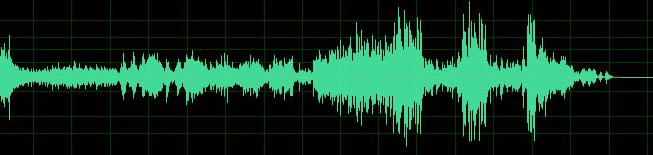
Fig. 1. Oscillogram sound
This is an oscillogram of sound - this is what an audio signal looks like. I think everyone has ever seen such pictures in their lives. In order to understand how the process of converting an analog signal to a digital one works, you need to draw a sound waveform on graph paper. For each vertical line, we find the point of intersection with the waveform and the nearest integer value on the vertical scale — a set of such values will be the simplest recording of a digital signal.
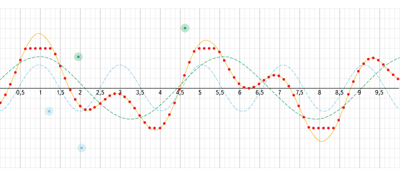
Fig. 2. An interactive example of adding waves and digitizing a signal.
Source: www.desmos.com/calculator/aojmanpjrl
We use this interactive example to understand how waves of different frequencies overlap and how digitization occurs. In the left menu, you can turn on / off the display of graphs, adjust the input data parameters and the sampling parameters, or you can simply move the control points.
At the hardware level, this , of course, looks much more complicated, and depending on the hardware, the signal can be encoded in completely different ways. The most common of these is pulse-code modulation , in which it is not the specific value of the signal level that is recorded at each point in time, but the difference between the current value and the previous value. This reduces the number of bits per sample by about 25%. This encoding method is used in the most common audio formats (WAV, MP3, WMA, OGG, FLAC, APE), which use the PCM WAV container.
In reality, to create a stereo effect when recording audio, most often not one, but several channels are recorded at once. Depending on the storage format used, they can be stored independently. Also, signal levels can be recorded as the difference between the level of the main channel and the level of the current one.
The inverse conversion from digital to analog is performed using digital-to-analog converters , which can have different devices and principles of operation. I will omit the description of these principles in this article.
As you know, a digital signal is a set of signal level values recorded at specified intervals. The process of converting a continuous analog signal to a digital signal is called discretization (by time and by level). There are two main characteristics of a digital signal - the sampling rate and the level of sampling depth.
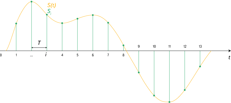
Fig. 3. Discrete signal.
Source: https://en.wikipedia.org/wiki/Sampling_(signal_processing)
The sampling rate indicates at what time intervals the data about the signal level go. There is a Kotelnikov theorem (in Western literature it is referred to as the Nyquist – Shannon theorem , although the name of Kotelnikov – Shannon is also found), which states that to be able to accurately reconstruct an analog signal from a discrete one, it is necessary that the sampling frequency be at least twice as high as in the analog signal. If we take an approximate range of human-perceived audio frequencies of 20 Hz - 20 kHz, then the optimal sampling frequency ( Nyquist frequency ) should be around 40 kHz. With standard audio CDs, it is 44.1 kHz.
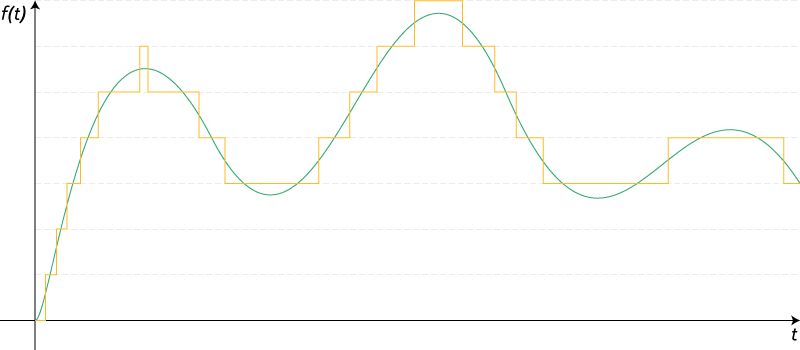
Fig. 4. Quantization of the signal.
Source: https://ru.wikipedia.org/wiki/ Quantization_ (signal processing)
The depth of sampling describes the digit capacity of the number, which describes the signal level. This characteristic imposes a limit on the accuracy of the signal level recording and on its minimum value. It should be specially noted that this characteristic is not related to loudness - it reflects the accuracy of the signal recording. The standard audio-CD sample rate is 16 bits. At the same time, if you do not use special studio equipment, most people no longer notice the difference in sound in the region of 10-12 bits. However, a large depth of sampling allows you to avoid the appearance of noise in the further processing of sound.
There are three main sources of noise in digital sound.
These are random deviations of a signal, as a rule, arising from the instability of the frequency of the master oscillator or different propagation speeds of different frequency components of one signal. This problem occurs at the digitization stage. If we describe“on the fingers” “on the graph paper”, this is due to the slightly different distance between the vertical lines.
It is directly related to the depth of sampling. Since when digitizing a signal, its real values are rounded off with a certain accuracy, there are weak noises associated with its loss. These noises can appear not only at the digitization stage, but also in the process of digital processing (for example, if the signal level is lowered first and then rises again).
When digitizing, a situation is possible in which frequency components may appear in a digital signal that were not in the original signal. This error is called Aliasing . This effect is directly related to the sampling frequency, and more precisely to the Nyquist frequency. The easiest way to understand how this happens is to look at this picture:
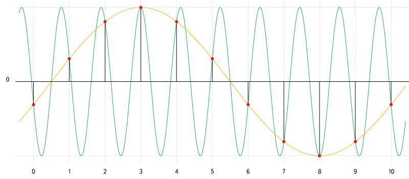
Fig. 5. Alias. Source: en.wikipedia.org/wiki/Aliassing
Green shows the frequency component, the frequency of which is higher than the Nyquist frequency. When digitizing such a frequency component, it is not possible to write enough data to correctly describe it. As a result, a completely different signal is produced during playback - a yellow curve.
For a start, it is worthwhile to immediately understand that when it comes to a digital signal, one can only speak of the relative signal level. The absolute depends primarily on the reproducing apparatus and is directly proportional to the relative. When calculating the relative signal levels, it is common to use decibels . In this case, the signal with the maximum possible amplitude at a given sampling depth is taken as a reference point. This level is indicated as 0 dBFS (dB - decibels, FS = Full Scale - full scale). Lower signal levels are indicated as -1 dBFS, -2 dBFS, etc. It is quite obvious that higher levels simply do not happen (we initially take the highest possible level).
At first it can be hard to figure out how the decibels correlate with the actual signal level. In fact, everything is simple. Every ~ 6 dB (more precisely, 20 log (2) ~ 6.02 dB) indicates a change in the signal level twice. That is, when we talk about a signal with a level of -12 dBFS, we understand that this is a signal whose level is four times less than the maximum, and -18 dBFS - at eight, and so on. If you look at the definition of decibel, it indicates the value) - then where does 20 come from? The thing is that the decibel is the logarithm of the ratio of two energy values of the same name multiplied by 10. The amplitude is not an energy value, therefore it must be converted to a suitable value. The power carried by waves with different amplitudes is proportional to the square of the amplitude. Therefore, for amplitude (if all other conditions, except amplitude, are assumed to be unchanged), the formula can be written as
- then where does 20 come from? The thing is that the decibel is the logarithm of the ratio of two energy values of the same name multiplied by 10. The amplitude is not an energy value, therefore it must be converted to a suitable value. The power carried by waves with different amplitudes is proportional to the square of the amplitude. Therefore, for amplitude (if all other conditions, except amplitude, are assumed to be unchanged), the formula can be written as %20%3D>%2020%20log(a%2Fa_0))
NB It is worth mentioning that the logarithm in this case is taken as a decimal, while the majority of libraries under the function called log implies the natural logarithm.
With different sampling depths, the signal level on this scale will not change. A signal with a level of -6 dBFS will remain a signal with a level of -6 dBFS. Yet one characteristic will change - the dynamic range. The dynamic range of a signal is the difference between its minimum and maximum value. It is calculated by the formula) where n is the sampling depth (for rough estimates, you can use a simpler formula: n * 6). For 16 bits this is ~ 96.33 dB, for 24 bits ~ 144.49 dB. This means that the largest level difference that can be described with a 24-bit sampling depth (144.49 dB) is 48.16 dB more than the largest level difference with 16-bit depth (96.33 dB). Plus, the crushing noise at 24 bits is 48 dB quieter.
where n is the sampling depth (for rough estimates, you can use a simpler formula: n * 6). For 16 bits this is ~ 96.33 dB, for 24 bits ~ 144.49 dB. This means that the largest level difference that can be described with a 24-bit sampling depth (144.49 dB) is 48.16 dB more than the largest level difference with 16-bit depth (96.33 dB). Plus, the crushing noise at 24 bits is 48 dB quieter.
When we talk about the perception of sound by man, we must first understand how people perceive sound. Obviously, we hear with the help of ears . Sound waves interact with the eardrum, displacing it. Vibrations are transmitted to the inner ear, where they are captured by receptors. How much the eardrum shifts depends on characteristics such as sound pressure . In this case, the perceived volume depends not directly, but logarithmically, on the sound pressure. Therefore, when changing the volume, it is customary to use the relative SPL scale (sound pressure level), the values of which are specified in the same decibels. It should also be noted that the perceived loudness of the sound depends not only on the sound pressure level, but also on the frequency of the sound:
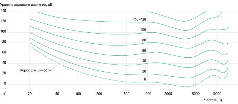
Fig. 6. Dependence of perceived volume on the frequency and amplitude of sound.
Source: ru.wikipedia.org/wiki/Sound_Sound
The simplest example of sound processing is changing its volume. When this happens, the signal level is simply multiplied by some fixed value. However, even in such a simple matter as volume control, there is one pitfall. As I noted earlier, the perceived volume depends on the logarithm of the sound pressure, which means that the use of a linear volume scale is not very effective. With a linear loudness scale, two problems arise at once - for a noticeable change in loudness, when the slider is above the middle of the scale, you have to move it far enough, while shifting closer to the very bottom of the scale is less than the thickness of the hair, it can change the volume twice everyone came across this). To solve this problem, a logarithmic volume scale is used. At the same time, throughout its entire length, moving the slider to a fixed distance changes the volume by the same number of times. In professional recording and processing equipment, as a rule, it is the logarithmic volume scale that is used.
Here I’ll probably get back to mathematics a bit, because the implementation of the logarithmic scale is not so simple and obvious thing for many, and finding this formula on the Internet is not as easy as I would like. At the same time I will show how easy it is to convert the volume values to dBFS and back. For further explanation, this will be helpful.
Now back to the fact that we have a digital rather than an analog signal. The digital signal has two features that should be considered when working with volume:
From the fact that the signal level has an accuracy limit, two things follow:
From the fact that the signal has an upper level limit, it follows that it is impossible to safely increase the volume above one. In this case, the peaks that will be above the boundary, will be "cut off" and there will be data loss.
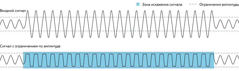
Fig. 7. Clipping.
Source: https://en.wikipedia.org/wiki/Clipping_(audio)
In practice, all this means that the standard for Audio-CD sampling parameters (16 bits, 44.1 kHz) do not allow for high-quality sound processing, because they have very little redundancy. For these purposes it is better to use more redundant formats. However, it should be borne in mind that the total file size is proportional to the discretization parameters, therefore issuing such files for online playback is not the best idea.
In order to compare the volume of two different signals, you first need to somehow measure it. There are at least three metrics for measuring the volume of the signals — the maximum peak value, the average value of the signal level, and the ReplayGain metric.
The maximum peak value is a fairly weak metric for estimating loudness. It does not take into account the overall volume level - for example, if you record a thunderstorm, then the rain will rustle quietly most of the time on the recording and only a few thunder will roar. The maximum peak value of the signal level of such a recording will be quite high, but most of the recording will have a very low signal level. However, this metric is still useful - it allows you to calculate the maximum gain that can be applied to the recording, at which there will be no data loss due to “clipping” the peaks.
The average signal level is a more useful metric and easily computable, but it still has significant drawbacks related to how we perceive sound. The screech of a circular saw and the roar of a waterfall, recorded with the same average signal level, will be perceived in completely different ways.
ReplayGain most accurately conveys the perceived volume of the recording and takes into account the physiological and mental characteristics of sound perception. For the industrial release of recordings, many recording studios use it, and it is also supported by most popular media players. (The Russian article on WIKI contains many inaccuracies and in fact does not correctly describe the very essence of the technology)
If we can measure the volume of different recordings, we can normalize it. The idea of normalization is to bring different sounds to the same level of perceived volume. For this, several different approaches are used. As a rule, they try to maximize the volume, but this is not always possible due to the limitations of the maximum signal level. Therefore, usually a certain value is taken that is slightly less than the maximum (for example, -14 dBFS), to which all signals are trying to lead.
Sometimes loudness normalization is carried out within the framework of a single recording - with the different parts of the recording being amplified by different values so that their perceived loudness is the same. This approach is very often used in computer video players - the soundtrack of many films may contain sections with very different loudness. In such a situation, there are problems when watching movies without headphones at a later time — with the volume at which the whispering of the main characters is normally heard, shots can wake up the neighbors. And at the volume, at which shots do not hit the ears, the whisper becomes generally indistinguishable. When in-track volume normalization, the player automatically increases the volume on quiet areas and lowers on loud ones. However, this approach creates tangible playback artifacts during abrupt transitions between a quiet and loud sound, and also sometimes overestimates the volume of some sounds, which should be background and barely distinguishable.
Also, internal normalization is sometimes performed to increase the overall volume of the tracks. This is called normalization with compression. With this approach, the average value of the signal level is maximized by increasing the entire signal by a specified amount. Those areas that should have been subjected to "circumcision", due to exceeding the maximum level, are amplified by a smaller amount, allowing you to avoid it. This way to increase the volume significantly reduces the sound quality of the track, but, nevertheless, many recording studios do not hesitate to use it.
I will not describe all the audio filters at all, I will limit myself to the standard ones that are present in the Web Audio API. The simplest and most common of these is the bi-square filter ( BiquadFilterNode ) - this is a second-order active filter with an infinite impulse response that can reproduce a fairly large number of effects. The principle of operation of this filter is based on the use of two buffers, each with two samples. One buffer contains the last two samples in the input signal, the other - the last two samples in the output signal. The resulting value is obtained by summing five values: the current sample and samples from both buffers multiplied by the previously calculated coefficients. The coefficients of this filter are not set directly, but are calculated from the parameters of frequency, quality factor (Q) and gain.
All graphs below display the frequency range from 20 Hz to 20,000 Hz. The horizontal axis displays the frequency, the logarithmic scale is applied along it, the vertical axis shows the magnitude (yellow graph) from 0 to 2, or the phase shift (green graph) from -Pi to Pi. The frequency of all filters (632 Hz) is marked with a red line on the graph.
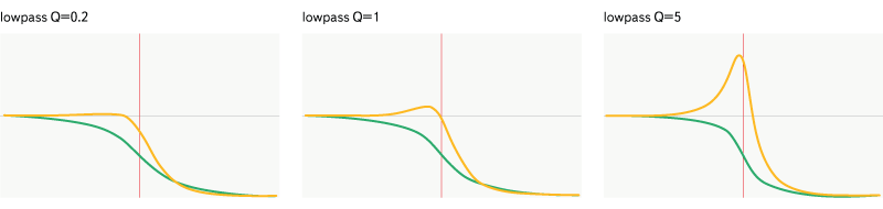
Fig. 8. Filter lowpass.
Only passes frequencies below the set frequency. The filter is set by frequency and quality.
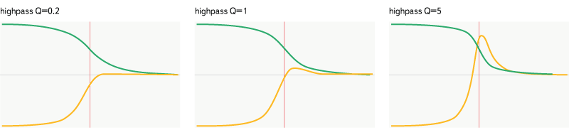
Fig. 9. Highpass filter.
It operates in the same way as lowpass, except for the fact that it skips frequencies higher than the specified one and not lower.
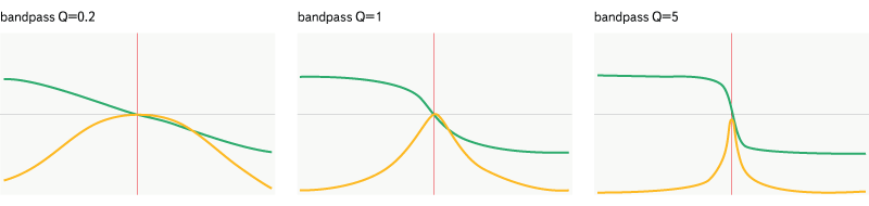
Fig. 10. Filter bandpass.
This filter is more selective - it passes only a certain frequency band.
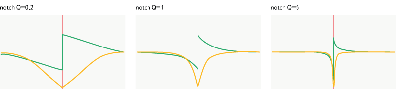
Fig. 11. Filter notch.
Is the opposite of bandpass - skips all frequencies outside the specified band. It is worth noting, however, the difference in the attenuation plots of the effects and in the phase characteristics of these filters.
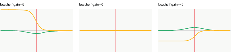
Fig. 12. Filter lowshelf.
It is a more "smart" version of highpass - strengthens or weakens the frequencies below the set, skips the frequencies above without changes. The filter is set by frequency and gain.
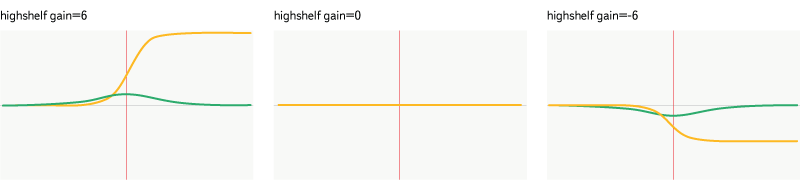
Fig. 13. Filter highshelf.
The smarter version of lowpass - strengthens or weakens the frequencies above the setpoint, passes the frequency below unchanged.
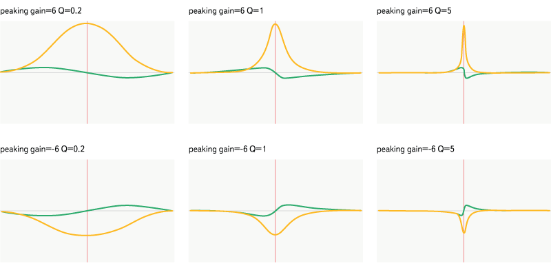
Fig. 14. Filter peaking.
This is a more “clever” version of notch - it strengthens or weakens the frequencies in a given range and skips the other frequencies without changes. The filter is set by frequency, gain and quality.
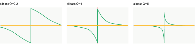
Fig. 15. Filter allpass.
Allpass is different from all the others - it does not change the amplitude characteristics of the signal, instead of which it does the phase shift of the specified frequencies. The filter is set by frequency and quality.
Wave Shaper ( en ) is used to create complex effects of sound distortion, in particular with the help of it you can realize the effects of distortion , overdrive and fuzz . This filter applies a special shaping function to the input signal. The principles of constructing such functions are quite complex and pull into a separate article, so I will omit their description.
A filter that produces a linear convolution of the input signal with an audio buffer that gives a certain impulse response . Impulse response is the answer of a certain system to a single impulse. In simple terms, this can be called a “photo” of sound. If a real photo contains information about light waves, about how much they are reflected, absorbed and interact, then the impulse response contains similar information about sound waves. Convolution of an audio stream with a similar “photo” seems to impose the effects of the environment in which the impulse response was taken on the input signal.
For the operation of this filter requires the decomposition of the signal into frequency components. This decomposition is performed using the fast Fourier transform (unfortunately, in the Russian-language Wikipedia a completely non-substantive article written, apparently, for people who already know what an FFT is and can themselves write the same non-substantive article). As I said in the introduction, I will not give the FFT mathematics in this article, but not to mention the cornerstone algorithm for digital signal processing would be wrong.
This filter has a reverb effect. There are many libraries of audio buffers for this filter that implement various effects ( 1 , 2 ), such libraries are well located on request [impulse response mp3].
Many thanks to my colleagues who helped collect materials for this article and gave useful advice.
Special thanks to Taras Audiophile Kovrizhenko for the description of the algorithms for the normalization and maximization of loudness and Sergei forgotten Konstantinov for a large number of explanations and tips on this article.
UPD. Corrected the section about filtering and added links for different types of filters. Thanks to Denis deniskreshikhin Kreschina and Nikita merlin-vrn Kipriyanov for paying attention.
To work on Yandex.Music, it is always important for us to remember about the different intricacies that sound harbors. What is loudness, how does it change and what does it depend on? How do sound filters work? What are the noises? How does the sound change? How people perceive it.
')
We learned quite a lot about all this while working on our project, and today I will try to describe on my fingers some basic concepts that you need to know if you are dealing with digital audio processing. This article does not have serious mathematics like fast Fourier transforms and so on — these formulas are easy to find on the web. I will describe the essence and meaning of the things that I have to face.
The reason for this post is that we have added the ability to listen to high-quality tracks (320kbps) to the Yandex.Music applications . And you can not count. So.
Digitization, or There and back
First of all, let us deal with what a digital signal is, how it is obtained from the analog signal, and where the analog signal is actually taken from. The latter can be as simply as possible defined as voltage fluctuations arising due to membrane oscillations in a microphone.
Fig. 1. Oscillogram sound
This is an oscillogram of sound - this is what an audio signal looks like. I think everyone has ever seen such pictures in their lives. In order to understand how the process of converting an analog signal to a digital one works, you need to draw a sound waveform on graph paper. For each vertical line, we find the point of intersection with the waveform and the nearest integer value on the vertical scale — a set of such values will be the simplest recording of a digital signal.
Fig. 2. An interactive example of adding waves and digitizing a signal.
Source: www.desmos.com/calculator/aojmanpjrl
We use this interactive example to understand how waves of different frequencies overlap and how digitization occurs. In the left menu, you can turn on / off the display of graphs, adjust the input data parameters and the sampling parameters, or you can simply move the control points.
At the hardware level, this , of course, looks much more complicated, and depending on the hardware, the signal can be encoded in completely different ways. The most common of these is pulse-code modulation , in which it is not the specific value of the signal level that is recorded at each point in time, but the difference between the current value and the previous value. This reduces the number of bits per sample by about 25%. This encoding method is used in the most common audio formats (WAV, MP3, WMA, OGG, FLAC, APE), which use the PCM WAV container.
In reality, to create a stereo effect when recording audio, most often not one, but several channels are recorded at once. Depending on the storage format used, they can be stored independently. Also, signal levels can be recorded as the difference between the level of the main channel and the level of the current one.
The inverse conversion from digital to analog is performed using digital-to-analog converters , which can have different devices and principles of operation. I will omit the description of these principles in this article.
Sampling
As you know, a digital signal is a set of signal level values recorded at specified intervals. The process of converting a continuous analog signal to a digital signal is called discretization (by time and by level). There are two main characteristics of a digital signal - the sampling rate and the level of sampling depth.
Fig. 3. Discrete signal.
Source: https://en.wikipedia.org/wiki/Sampling_(signal_processing)
The sampling rate indicates at what time intervals the data about the signal level go. There is a Kotelnikov theorem (in Western literature it is referred to as the Nyquist – Shannon theorem , although the name of Kotelnikov – Shannon is also found), which states that to be able to accurately reconstruct an analog signal from a discrete one, it is necessary that the sampling frequency be at least twice as high as in the analog signal. If we take an approximate range of human-perceived audio frequencies of 20 Hz - 20 kHz, then the optimal sampling frequency ( Nyquist frequency ) should be around 40 kHz. With standard audio CDs, it is 44.1 kHz.
Fig. 4. Quantization of the signal.
Source: https://ru.wikipedia.org/wiki/ Quantization_ (signal processing)
The depth of sampling describes the digit capacity of the number, which describes the signal level. This characteristic imposes a limit on the accuracy of the signal level recording and on its minimum value. It should be specially noted that this characteristic is not related to loudness - it reflects the accuracy of the signal recording. The standard audio-CD sample rate is 16 bits. At the same time, if you do not use special studio equipment, most people no longer notice the difference in sound in the region of 10-12 bits. However, a large depth of sampling allows you to avoid the appearance of noise in the further processing of sound.
Noises
There are three main sources of noise in digital sound.
Jitter
These are random deviations of a signal, as a rule, arising from the instability of the frequency of the master oscillator or different propagation speeds of different frequency components of one signal. This problem occurs at the digitization stage. If we describe
Crushing noise
It is directly related to the depth of sampling. Since when digitizing a signal, its real values are rounded off with a certain accuracy, there are weak noises associated with its loss. These noises can appear not only at the digitization stage, but also in the process of digital processing (for example, if the signal level is lowered first and then rises again).
Aliasing
When digitizing, a situation is possible in which frequency components may appear in a digital signal that were not in the original signal. This error is called Aliasing . This effect is directly related to the sampling frequency, and more precisely to the Nyquist frequency. The easiest way to understand how this happens is to look at this picture:
Fig. 5. Alias. Source: en.wikipedia.org/wiki/Aliassing
Green shows the frequency component, the frequency of which is higher than the Nyquist frequency. When digitizing such a frequency component, it is not possible to write enough data to correctly describe it. As a result, a completely different signal is produced during playback - a yellow curve.
Signal strength
For a start, it is worthwhile to immediately understand that when it comes to a digital signal, one can only speak of the relative signal level. The absolute depends primarily on the reproducing apparatus and is directly proportional to the relative. When calculating the relative signal levels, it is common to use decibels . In this case, the signal with the maximum possible amplitude at a given sampling depth is taken as a reference point. This level is indicated as 0 dBFS (dB - decibels, FS = Full Scale - full scale). Lower signal levels are indicated as -1 dBFS, -2 dBFS, etc. It is quite obvious that higher levels simply do not happen (we initially take the highest possible level).
At first it can be hard to figure out how the decibels correlate with the actual signal level. In fact, everything is simple. Every ~ 6 dB (more precisely, 20 log (2) ~ 6.02 dB) indicates a change in the signal level twice. That is, when we talk about a signal with a level of -12 dBFS, we understand that this is a signal whose level is four times less than the maximum, and -18 dBFS - at eight, and so on. If you look at the definition of decibel, it indicates the value
NB It is worth mentioning that the logarithm in this case is taken as a decimal, while the majority of libraries under the function called log implies the natural logarithm.
With different sampling depths, the signal level on this scale will not change. A signal with a level of -6 dBFS will remain a signal with a level of -6 dBFS. Yet one characteristic will change - the dynamic range. The dynamic range of a signal is the difference between its minimum and maximum value. It is calculated by the formula
Perception
When we talk about the perception of sound by man, we must first understand how people perceive sound. Obviously, we hear with the help of ears . Sound waves interact with the eardrum, displacing it. Vibrations are transmitted to the inner ear, where they are captured by receptors. How much the eardrum shifts depends on characteristics such as sound pressure . In this case, the perceived volume depends not directly, but logarithmically, on the sound pressure. Therefore, when changing the volume, it is customary to use the relative SPL scale (sound pressure level), the values of which are specified in the same decibels. It should also be noted that the perceived loudness of the sound depends not only on the sound pressure level, but also on the frequency of the sound:
Fig. 6. Dependence of perceived volume on the frequency and amplitude of sound.
Source: ru.wikipedia.org/wiki/Sound_Sound
Volume
The simplest example of sound processing is changing its volume. When this happens, the signal level is simply multiplied by some fixed value. However, even in such a simple matter as volume control, there is one pitfall. As I noted earlier, the perceived volume depends on the logarithm of the sound pressure, which means that the use of a linear volume scale is not very effective. With a linear loudness scale, two problems arise at once - for a noticeable change in loudness, when the slider is above the middle of the scale, you have to move it far enough, while shifting closer to the very bottom of the scale is less than the thickness of the hair, it can change the volume twice everyone came across this). To solve this problem, a logarithmic volume scale is used. At the same time, throughout its entire length, moving the slider to a fixed distance changes the volume by the same number of times. In professional recording and processing equipment, as a rule, it is the logarithmic volume scale that is used.
Maths
Here I’ll probably get back to mathematics a bit, because the implementation of the logarithmic scale is not so simple and obvious thing for many, and finding this formula on the Internet is not as easy as I would like. At the same time I will show how easy it is to convert the volume values to dBFS and back. For further explanation, this will be helpful.
// - var EPSILON = 0.001; // dBFS var DBFS_COEF = 20 / Math.log(10); // var volumeToExponent = function(value) { var volume = Math.pow(EPSILON, 1 - value); return volume > EPSILON ? volume : 0; }; // var volumeFromExponent = function(volume) { return 1 - Math.log(Math.max(volume, EPSILON)) / Math.log(EPSILON); }; // dBFS var volumeToDBFS = function(volume) { return Math.log(volume) * DBFS_COEF; }; // dBFS var volumeFromDBFS = function(dbfs) { return Math.exp(dbfs / DBFS_COEF); } Digital processing
Now back to the fact that we have a digital rather than an analog signal. The digital signal has two features that should be considered when working with volume:
- the accuracy with which the signal level is indicated is limited (and strong enough. 16 bit is 2 times less than that used for a standard floating point number);
- the signal has an upper limit of the level beyond which it cannot reach.
From the fact that the signal level has an accuracy limit, two things follow:
- crushing noise level increases with increasing volume. For small changes, this is usually not very critical, since the initial noise level is much quieter than perceptible, and it can be safely raised 4-8 times (for example, use an equalizer with a scale limit of ± 12dB);
- you should not first strongly lower the signal level, and then greatly increase it - at the same time, new crushing noises may appear, which were not there initially.
From the fact that the signal has an upper level limit, it follows that it is impossible to safely increase the volume above one. In this case, the peaks that will be above the boundary, will be "cut off" and there will be data loss.
Fig. 7. Clipping.
Source: https://en.wikipedia.org/wiki/Clipping_(audio)
In practice, all this means that the standard for Audio-CD sampling parameters (16 bits, 44.1 kHz) do not allow for high-quality sound processing, because they have very little redundancy. For these purposes it is better to use more redundant formats. However, it should be borne in mind that the total file size is proportional to the discretization parameters, therefore issuing such files for online playback is not the best idea.
Volume measurement
In order to compare the volume of two different signals, you first need to somehow measure it. There are at least three metrics for measuring the volume of the signals — the maximum peak value, the average value of the signal level, and the ReplayGain metric.
The maximum peak value is a fairly weak metric for estimating loudness. It does not take into account the overall volume level - for example, if you record a thunderstorm, then the rain will rustle quietly most of the time on the recording and only a few thunder will roar. The maximum peak value of the signal level of such a recording will be quite high, but most of the recording will have a very low signal level. However, this metric is still useful - it allows you to calculate the maximum gain that can be applied to the recording, at which there will be no data loss due to “clipping” the peaks.
The average signal level is a more useful metric and easily computable, but it still has significant drawbacks related to how we perceive sound. The screech of a circular saw and the roar of a waterfall, recorded with the same average signal level, will be perceived in completely different ways.
ReplayGain most accurately conveys the perceived volume of the recording and takes into account the physiological and mental characteristics of sound perception. For the industrial release of recordings, many recording studios use it, and it is also supported by most popular media players. (The Russian article on WIKI contains many inaccuracies and in fact does not correctly describe the very essence of the technology)
Volume normalization
If we can measure the volume of different recordings, we can normalize it. The idea of normalization is to bring different sounds to the same level of perceived volume. For this, several different approaches are used. As a rule, they try to maximize the volume, but this is not always possible due to the limitations of the maximum signal level. Therefore, usually a certain value is taken that is slightly less than the maximum (for example, -14 dBFS), to which all signals are trying to lead.
Sometimes loudness normalization is carried out within the framework of a single recording - with the different parts of the recording being amplified by different values so that their perceived loudness is the same. This approach is very often used in computer video players - the soundtrack of many films may contain sections with very different loudness. In such a situation, there are problems when watching movies without headphones at a later time — with the volume at which the whispering of the main characters is normally heard, shots can wake up the neighbors. And at the volume, at which shots do not hit the ears, the whisper becomes generally indistinguishable. When in-track volume normalization, the player automatically increases the volume on quiet areas and lowers on loud ones. However, this approach creates tangible playback artifacts during abrupt transitions between a quiet and loud sound, and also sometimes overestimates the volume of some sounds, which should be background and barely distinguishable.
Also, internal normalization is sometimes performed to increase the overall volume of the tracks. This is called normalization with compression. With this approach, the average value of the signal level is maximized by increasing the entire signal by a specified amount. Those areas that should have been subjected to "circumcision", due to exceeding the maximum level, are amplified by a smaller amount, allowing you to avoid it. This way to increase the volume significantly reduces the sound quality of the track, but, nevertheless, many recording studios do not hesitate to use it.
Filtration
I will not describe all the audio filters at all, I will limit myself to the standard ones that are present in the Web Audio API. The simplest and most common of these is the bi-square filter ( BiquadFilterNode ) - this is a second-order active filter with an infinite impulse response that can reproduce a fairly large number of effects. The principle of operation of this filter is based on the use of two buffers, each with two samples. One buffer contains the last two samples in the input signal, the other - the last two samples in the output signal. The resulting value is obtained by summing five values: the current sample and samples from both buffers multiplied by the previously calculated coefficients. The coefficients of this filter are not set directly, but are calculated from the parameters of frequency, quality factor (Q) and gain.
All graphs below display the frequency range from 20 Hz to 20,000 Hz. The horizontal axis displays the frequency, the logarithmic scale is applied along it, the vertical axis shows the magnitude (yellow graph) from 0 to 2, or the phase shift (green graph) from -Pi to Pi. The frequency of all filters (632 Hz) is marked with a red line on the graph.
Lowpass
Fig. 8. Filter lowpass.
Only passes frequencies below the set frequency. The filter is set by frequency and quality.
Highpass
Fig. 9. Highpass filter.
It operates in the same way as lowpass, except for the fact that it skips frequencies higher than the specified one and not lower.
Bandpass
Fig. 10. Filter bandpass.
This filter is more selective - it passes only a certain frequency band.
Notch
Fig. 11. Filter notch.
Is the opposite of bandpass - skips all frequencies outside the specified band. It is worth noting, however, the difference in the attenuation plots of the effects and in the phase characteristics of these filters.
Lowshelf
Fig. 12. Filter lowshelf.
It is a more "smart" version of highpass - strengthens or weakens the frequencies below the set, skips the frequencies above without changes. The filter is set by frequency and gain.
Highshelf
Fig. 13. Filter highshelf.
The smarter version of lowpass - strengthens or weakens the frequencies above the setpoint, passes the frequency below unchanged.
Peaking
Fig. 14. Filter peaking.
This is a more “clever” version of notch - it strengthens or weakens the frequencies in a given range and skips the other frequencies without changes. The filter is set by frequency, gain and quality.
Allpass filter
Fig. 15. Filter allpass.
Allpass is different from all the others - it does not change the amplitude characteristics of the signal, instead of which it does the phase shift of the specified frequencies. The filter is set by frequency and quality.
Filter WaveShaperNode
Wave Shaper ( en ) is used to create complex effects of sound distortion, in particular with the help of it you can realize the effects of distortion , overdrive and fuzz . This filter applies a special shaping function to the input signal. The principles of constructing such functions are quite complex and pull into a separate article, so I will omit their description.
ConvolverNode filter
A filter that produces a linear convolution of the input signal with an audio buffer that gives a certain impulse response . Impulse response is the answer of a certain system to a single impulse. In simple terms, this can be called a “photo” of sound. If a real photo contains information about light waves, about how much they are reflected, absorbed and interact, then the impulse response contains similar information about sound waves. Convolution of an audio stream with a similar “photo” seems to impose the effects of the environment in which the impulse response was taken on the input signal.
For the operation of this filter requires the decomposition of the signal into frequency components. This decomposition is performed using the fast Fourier transform (unfortunately, in the Russian-language Wikipedia a completely non-substantive article written, apparently, for people who already know what an FFT is and can themselves write the same non-substantive article). As I said in the introduction, I will not give the FFT mathematics in this article, but not to mention the cornerstone algorithm for digital signal processing would be wrong.
This filter has a reverb effect. There are many libraries of audio buffers for this filter that implement various effects ( 1 , 2 ), such libraries are well located on request [impulse response mp3].
Materials
- On the concept of loudness in the digital representation of sound and on the methods of its increase
- Sound
- Amplitude
- Frequency
- Digital signal
- Analog signal
- Digital signal processing
- Interactive example of wave addition and signal digitization
- Analog-to-digital converter
- D / A converter
- Pulse code modulation
- PCM WAV format
- Sampling (en)
- Sampling frequency
- Kotelnikov theorem
- Nyquist frequency
- Sampling depth
- Alias
- Decibel
- Ear structure
- Sound pressure
- Perceived volume
- Clipping
- ReplayGain Description
- ReplayGain specification
- Fast Fourier transform , wiki , wiki
- Impulse response
- Phase Frequency Response
- Amplitude-frequency response
- Infinite impulse response filter
- Filter with finite impulse response
- Bi-Square Filter (en)
- BiquadFilterNode
- HTML5 Audio W3C
- Web Audio API
- Waveshaper
- Distortion
- Overdrive
- Fuzz
- Reverb
- Convolution
- Equalizer
Many thanks to my colleagues who helped collect materials for this article and gave useful advice.
Special thanks to Taras Audiophile Kovrizhenko for the description of the algorithms for the normalization and maximization of loudness and Sergei forgotten Konstantinov for a large number of explanations and tips on this article.
UPD. Corrected the section about filtering and added links for different types of filters. Thanks to Denis deniskreshikhin Kreschina and Nikita merlin-vrn Kipriyanov for paying attention.
Source: https://habr.com/ru/post/270765/
All Articles