How we teach machine learning and data analysis in Beeline

After a long preparation, selection of materials and preliminary approbations of the course, on October 19 we started. Corporate intensive practical course of data analysis from the experts of this case. At the moment we have 6 classes, half of our course, and this is a brief overview of what we do on them.

First of all, our task was to create a course in which we would give the maximum of practice that students could immediately apply in their daily work.
')
We often saw how people who came to us for interviews, despite their good knowledge of the theory, because of lack of experience could not reproduce all the stages of solving a typical machine learning task - data preparation, feature selection / design, model selection, their correct composition, achieving high quality and correct interpretation of the results.

Therefore, our main thing is practice. Open notebooks IPython and immediately work with them.

In the first lesson, we discussed the decision trees and forests and dismantled the feature extraction technique using the Kaggle Titanic: Machine Learning from Disaster data set as an example.

We believe that participation in machine learning competitions is necessary in order to maintain the required level and continually improve the analyst’s expertise. Therefore, starting from the first lesson, we launched our own car insurance payout competition (now a very popular topic in business) with the help of Kaggle Inclass. The competition will last until the end of the course.

In the second lesson, we analyzed Titanic data using Pandas and visualization tools. Also tried simple classification methods on the task of predicting payments in auto insurance.

In the third session, we considered the Kaggle “Greek Media Monitoring Multilabel Classification (WISE 2014)” task and the use of mixing algorithms as the main technique for most Kaggle competitions.

In the third lesson, we also looked at the capabilities of the Scikit-Learn machine learning library, and then more detailed linear classification methods: logistic regression and linear SVM, discussed when it is better to use linear models, and when complex ones. We talked about the importance of signs in the task of learning and on the quality metrics of classification.

The main topic of the fourth lesson was the meta-learning stacking algorithm and its application in Otto’s Kaggle winning solution to the Classification products into correct category.

In the fourth lesson, we got to the main problem of machine learning - the fight against retraining; we looked at how to use the learning and validation curves for this, how to cross-validate correctly, and what indicators can be optimized in this process to achieve the best generalizing ability. They also studied methods for constructing ensembles of classifiers and regressors — bagging, random subspaces, boosting, stacking, etc.

And so on - each lesson is a new practical task.

Since our main language on the course is Python, we are, of course, familiar with the main libraries of data analysis in the Python language — NumPy, SciPy, Matplotlib, Seaborn, Pandas, and Scikit-learn. We spend a lot of time on this, since the work of a data researcher largely consists of calling various methods of the listed modules.

Understanding the theory on which the methods are based is also important. Therefore, we considered the basic mathematical methods implemented in SciPy - finding eigenvalues, singular decomposition of the matrix, maximum likelihood method, optimization methods, etc. These methods were considered not just theoretically, but in conjunction with machine learning algorithms , logistic regression, spectral clustering, the method of principal components, etc. This approach is first practice, then theory, and finally, practice at a new level, with a theoretical understanding - p marketed by many machine learning schools abroad.

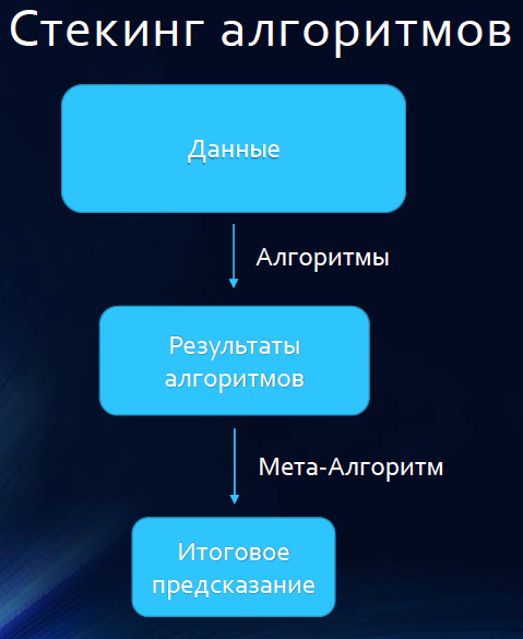
Let's take a closer look at one of the popular methods often used by participants in Kaggle competitions - stacking, which we studied in the fourth lesson.

In its simplest form, the idea of ​​stacking is to take M basic algorithms (for example, 10), split the training set into two parts - say, A and B. First, teach all M basic algorithms into part A and make predictions for part B. Then, on the contrary, train all models on part B and make predictions for objects from part A. This way, you can get a prediction matrix whose dimensions are nx M, where n is the number of objects in the original training set, M is the number of basic algorithms. This matrix is ​​fed to the input of another model - the model of the second level, which, in fact, is trained on learning outcomes.



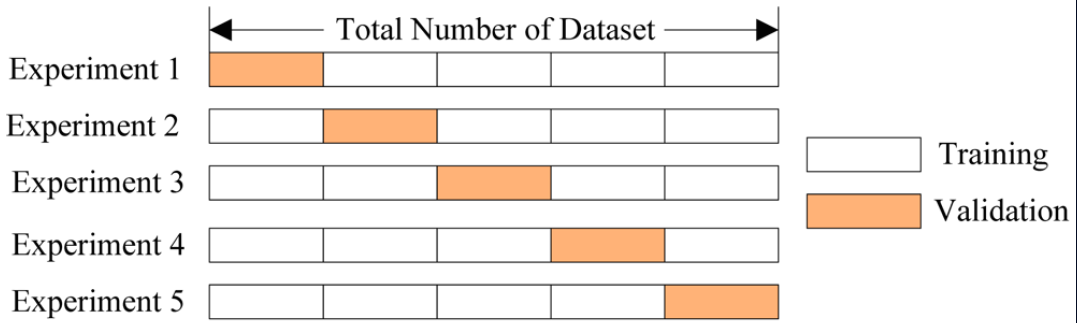
Often make the scheme a little more complicated. To train models on more data than half of the training sample, the sample is divided K times into K parts. Models are trained on the K-1 parts of the training sample, predictions are made on one part and bring the results into the matrix of predictions. This is a K-fold stacking.



Let us briefly review the winners of the Kaggle Otto Group Product Classification Challenge. www.kaggle.com/c/otto-group-product-classification-challenge
The task was to correctly classify goods into one of 9 categories based on 93 attributes, the essence of which Otto does not disclose. Predictions were estimated based on the average F1-measure. The competition became the most popular in the history of Kaggle, perhaps because the entry threshold was low, the data was well prepared, you could quickly take and try one of the models.

In deciding the winners of the competition, essentially the same K-fold stacking was used, only at the second level, three models were trained, not just one, and then the predictions of these three models were mixed.



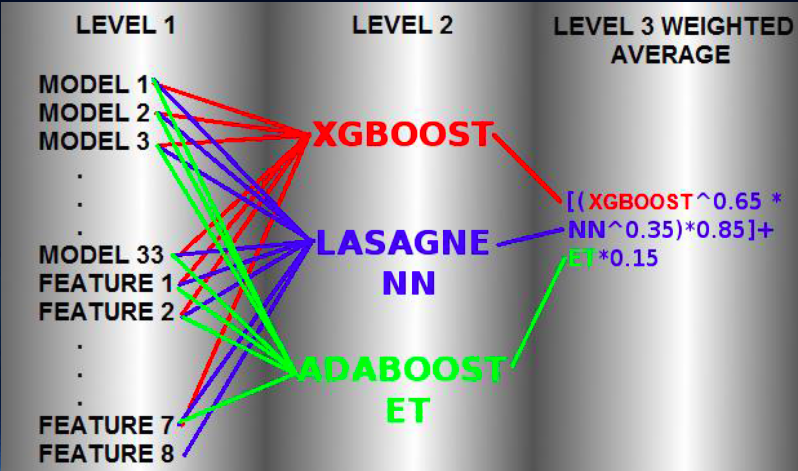
At the first level, 33 models were trained - various implementations of many machine learning algorithms with different sets of features, including those created.

These 33 models were trained 5 times in 80% of the training set and made predictions for the remaining 20% ​​of the data. The resulting predictions were collected in the matrix. That is, 5-fold stacking. But the difference from the classical stacking model is that the predictions of the 33 models were supplemented with 8 created features — mostly the initial data obtained by clustering the data (and the feature itself — labels of the received clusters) or taking into account the distances to the closest representatives of each class.

On the learning outcomes of 33 first-level models and 8 created features, 3 second-level models were trained - XGboost, Lasagne NN neural network and AdaBoost with ExtraTrees trees. The parameters of each algorithm were selected in the process of cross-validation. The final formula for averaging the predictions of models of the second level was also selected in the process of cross-validation.

In the fifth lesson, we continued to study the classification algorithms, namely, neural networks. They also touched upon the topic of learning without a teacher - clustering, reducing dimensions and searching for outliers.

In the sixth lesson, we plunged into Data Mining and an analysis of the consumer basket. It is widely believed that machine learning and data mining are the same or the latter is part of the first. We explain that this is not the case and point out the differences.

Initially, machine learning was more aimed at predicting the type of new objects based on the analysis of the training set, and the classification problem is most often remembered when people talk about machine learning.

The mining of data was focused on the search for “interesting” patterns (patterns) in the data, for example, of frequently purchased goods together. Of course, now this edge is being erased, and those methods of machine learning, which work not as a black box, but give out and interpreted rules, can be used to look for patterns.

So, the decision tree allows you to understand not only that this user behavior is similar to fraud, but why. Such rules resemble association rules, however, they appeared in mining data for analyzing sales, because it is useful to know that seemingly unrelated products are bought together. By purchasing A buy and B.

We not only talk about all this, but also give the opportunity to analyze the real data on such purchases. So data on sales of contextual advertising will help to understand what recommendations for the purchase of search phrases to give to those who want to promote their online store in the network.

Another important method for mining data is searching for frequent sequences. If the sequence <laminate, fridge> is quite frequent, then most likely you will buy new settlers in your store. And such sequences are useful for predicting the next purchases.

A separate lesson is devoted to recommender systems. We not only teach classical algorithms for collaborative filtering, but also dispel misconceptions that SVD, the de facto standard in this area, is a panacea for all recommender tasks. So, in the task of recommending radio stations, SVD is noticeably retrained, and the rather natural hybrid approach of collaborative filtering based on the similarity of users and dynamic profiles of users and radio stations based on tags works great.

So, six lessons passed, what next? Further more. We will have an analysis of social networks, we will build a recommendation system from scratch, teach processing and comparison of texts. Also, of course, we will have Big Data analysis using Apache Spark.

We will also give a separate lesson to tricks and tricks on Kaggle, about which a person who is now in 4th place in the world Kaggle rating will tell.

From November 16 we will launch the second course for those who could not get on the first one. Details, as usual, on bigdata.beeline.digital .

You can follow the chronicle of the current course on our Facebook page .