Some repositories to help learners and teachers of Python and machine learning.
Hello to the community!
I am Yuri Kashnitsky, I used to do a review of some MOOCs on computer science here and searched for “outliers” among Playboy models.
')
Now I teach Python and machine learning at the Faculty of Computer Science at HSE and in the online MLClass data analysis community course, as well as machine learning and big data analysis at a data school of one of the Russian telecom operators.
Why not Sunday evening to share with the community materials on Python and a review of machine learning repositories ... In the first part there will be a description of the GitHub repository with IPython notebooks on Python programming. The second is an example of course material “Machine Learning with Python”. In the third part, I will show one of the tricks used by the participants of the Kaggle competition, specifically, Stanislav Semenov (4th place in the current world rating of Kaggle). Finally, I'll review the cool GitHub repositories for programming, data analysis, and machine learning in Python.
Part 1. Python programming course in the form of IPython notebooks
The course consists of 5 lessons: a review of development tools, an introduction to the Python language, 2 lessons about data structures (Python and not only) and some algorithms and one lesson about functions and recursion. Yes, the topic of OOP and heaps of everything useful is not touched upon, but work on the course is under way, the repository will be updated.
The objectives of this course are:
- Learn the basics of the Python language
- Introduce the main data structures.
- Give the skills needed to develop simple algorithms
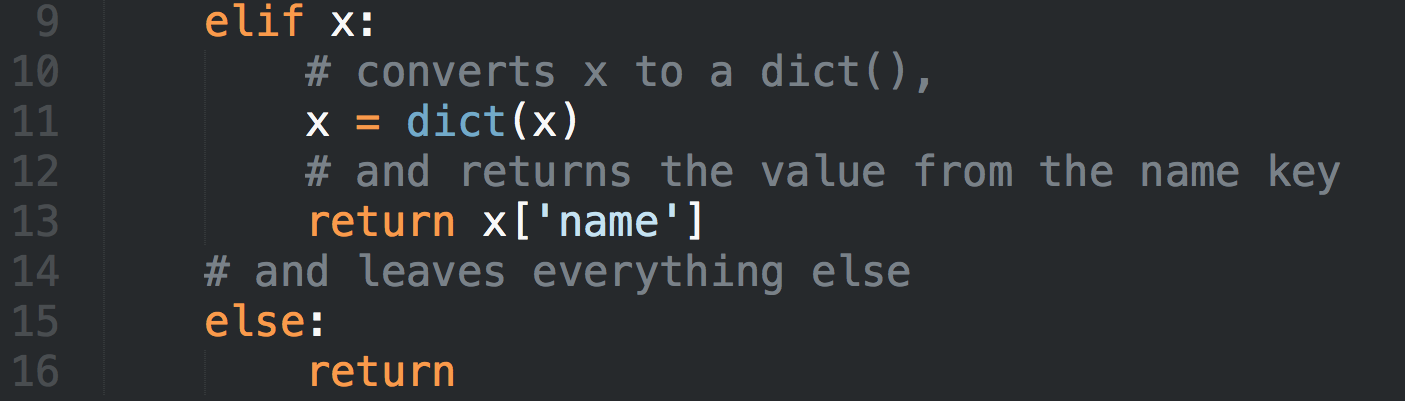
The IPython notebooks are chosen as the main means of presenting the material due to the fact that they can combine text, images, formulas and code. As a demonstration in the repository, a notebook about decision trees and their implementation in the Scikit-learn machine learning library is provided . The materials of the first lesson describe how to use these notebooks properly.

Here is a link to the GitHub repository with IPython notebooks. Branch and multiply, you can use for any purpose other than commercial, with reference to the author. If you want to connect to the project GitHub - write. You can report bugs in the materials.
Part 2. Example material for the course "Machine Learning with Python". Decision Trees
The course “Machine learning using Python” consists of 6 lessons and about 35 notebooks IPython about the basics of machine learning with the Scikit-learn library, using the NumPy, SciPy, Pandas libraries, with examples of solving real Kaggle problems and parsing practices used by the winners of Kaggle competitions - stacking, blending, ensembles of algorithms. Detailed program here . As an example of the presentation of the material consider one of the first topics - decision trees.
What is a decision tree?
We begin the review of classification methods, of course, with the most popular - decision tree.
Decision trees are used in everyday life in the most diverse areas of human activity, sometimes very far from machine learning. Decision tree can be called visual instruction what to do in what situation. Let us give an example from the field of consulting research institutes. The Higher School of Economics publishes info-schemes that make life easier for its employees. Here is a fragment of the instruction for publishing a scientific article on the institute portal.
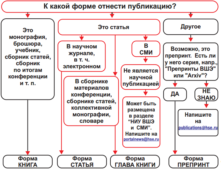
In terms of machine learning, we can say that this is an elementary classifier that determines the form of publication on the portal (book, article, chapter of the book, preprint, publication in “HSE and the media”) on several grounds - the type of publication (monograph, brochure, article and etc.), the type of publication in which the article was published (a scientific journal, a collection of papers, etc.) and the rest.
Often, a decision tree serves as a synthesis of expert experience, a means of transferring knowledge to future employees or a model of a company's business process. For example, prior to the introduction of scalable machine learning algorithms in the banking sector, the task of credit scoring was solved by experts. The decision to issue a loan to the borrower was made on the basis of some intuitively (or by experience) derived rules that can be represented as a decision tree.
In this case, we can say that the binary classification problem is being solved (the target class has two meanings - “Give out credit” and “Refuse”) according to the signs “Age”, “Household”, “Income” and “Education”.
The decision tree as an algorithm for machine learning is essentially the same, combining logical rules of the form “Characteristic value a is less than x And Characteristic value b is less than y ... => Class 1” into the data structure “Tree”. The tremendous advantage of decision trees is that they are easily interpretable, understandable to humans. For example, according to the scheme in Figure 2, the borrower can be explained why he was denied a loan. For example, because he does not have a home and the income is less than 5000. As we will see later, many other, albeit more accurate, models do not have this property and can rather be viewed as a “black box” into which they downloaded data and received a response. Due to this “clarity” of decision trees and their similarity to the model of decision making by a person (you can easily explain your model to the boss), decision trees have gained immense popularity, and one of the representatives of this group of classification methods, C4.5, is considered first in the list 10 best data mining algorithms (Top 10 algorithms in data mining, 2007).
How to build a decision tree
In the example of credit scoring, we saw that the decision to issue a loan was made on the basis of age, availability of real estate, income, and others. But which sign to choose first? To do this, consider an example more simply, where all the signs are binary.
Here you can recall the game “20 questions”, which is often mentioned in the introduction to decision trees. Surely everyone was playing it. One person makes a celebrity, and the second tries to guess by asking only questions that can be answered with “Yes” or “No” (omitting the options “I don’t know” and “I can’t say”). What question guesses ask the first thing? Of course, one that will reduce the number of remaining options the most. For example, the question “Is this Angelina Jolie?” In the case of a negative answer will leave more than 6 billion options for further searching (of course, less, not every person is a celebrity, but still a lot), but the question “Is this a woman?” half celebrities. That is, the sign of “sex” is much better shared by a sample of people than the sign of “this is Angelina Jolie”, “Spanish nationality” or “loves football”. This is intuitively consistent with the concept of information gain based on entropy.
Entropy
Shannon entropy is defined as
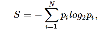
where N is the number of possible implementations, p_i (sorry, I didn’t bother with Habr's integration with TeX, it's time to deploy MathJax) - the probabilities of these implementations. This is a very important concept used in physics, information theory and other fields. Omitting the premises of the introduction (combinatorial and information-theoretic) of this concept, we note that, intuitively, entropy corresponds to the degree of chaos in the system. The higher the entropy, the less ordered the system and vice versa. This will help there to formalize the “effective division of the sample”, which we talked about in the context of the game “20 questions”.
Example
Consider a toy example in which we predict the color of the ball according to its coordinate. Of course, it has nothing to do with life, but it does allow showing how entropy is used to build a decision tree. Pictures are taken from this article.
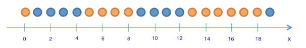
There are 9 blue balls and 11 yellow balls. If we pulled a ball at random, it will be blue with probability p1 = 9/20 and yellow with probability p2 = 11/20. This means that the state entropy is S0 = -9/20 log (9/20) -11/20 log (11/20) = ~ 1.
This value itself does not tell us anything yet.
Now let's see how the entropy changes, if the balls are divided into two groups - with a coordinate less than or equal to 12 and more than 12.
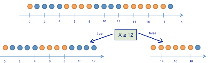
In the left group were 13 balls, of which 8 are blue and 5 are yellow. The entropy of this group is S1 = -5/13 log (5/13) -8/13 log (8/13) = ~ 0.96. In the right group were 7 balls, of which 1 is blue and 6 are yellow. The entropy of the right group is S2 = - 1/7 log (1/7) - 6/7 log (6/7) = ~ 0.6. As you can see, the entropy decreased in both groups as compared with the initial state, although not much in the left state. Since entropy is essentially a degree of chaos (or uncertainty) in a system, a decrease in entropy is called an increase in information. Formally, the information gain (information gain, IG) when dividing a sample on the basis of Q (in our example, it is “x <= 12”) is defined as
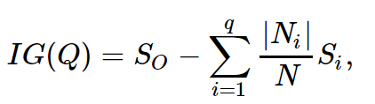
where q is the number of groups after splitting, N_i is the number of sample elements whose attribute Q has the i-th value. In our case, after separation, we got two groups (q = 2) —one of the 13 elements (N1 = 13), the second of 7 (N2 = 7). The increase in information turned out to be IG (“x <= 12”) = S0 - 13/20 S1 - 7/20 S2 = ~ 0.16.
It turns out that by dividing the balls into two groups on the basis of a “coordinate less or equal to 12”, we have already received a more ordered system than at the beginning. We continue the division of the balls into groups until the balls in each group are of the same color.
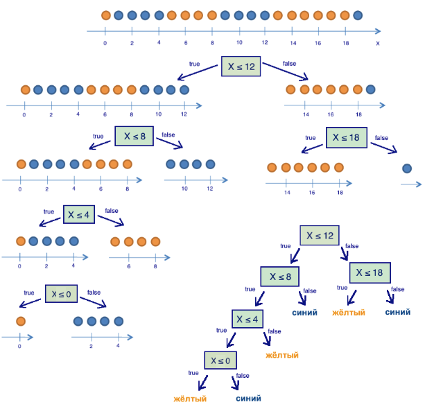
For the right group, it took only one additional splitting on the basis of “the coordinate is less or equal to 18” with the increase in information, for the left - three more. Obviously, the entropy of a group with balls of the same color is 0 (log (1) = 0), which corresponds to the idea that the group of balls of the same color is ordered. As a result, a decision tree was built, predicting the color of the ball according to its coordinate. Note that such a decision tree can work poorly for new objects (determining the color of new balls), since it ideally adjusted to the training sample (the original 20 balls). To classify new balls, a tree with a smaller number of “questions”, or divisions, is better suited, even if it does not ideally divide the training set by color. This problem, retraining, we will look further.
Tree building algorithm
One can make sure that the tree constructed in the previous example is in a certain sense optimal - it took only 5 “questions” (conditions for the x attribute) to “fit” the decision tree to the training set, that is, the tree correctly classified any learning object. Under other conditions of sampling separation, the tree will turn out deeper.
The basis of popular decision-making algorithms, such as ID3 and C4.5, is the principle of greedily maximizing the growth of information - at each step, the feature is chosen, when divided into which information growth is greatest. Then the procedure is repeated recursively until the entropy is zero or some small value (unless the tree is ideally fitted to the training set in order to avoid retraining). Different algorithms use different heuristics for “early stopping” or “clipping” to avoid building a retrained tree.
Example
Consider an example of using the decision tree from the Scikit-learn library for synthetic data.
%pylab inline import numpy as np import pylab as plt plt.rcParams['figure.figsize'] = (10.0, 8.0) Generate data. Two classes will be generated from two normal distributions with different means.
# train_data = np.random.normal(size=(100, 2)) train_labels = np.zeros(100) # train_data = np.r_[train_data, np.random.normal(size=(100, 2), loc=2)] train_labels = np.r_[train_labels, np.ones(100)] We will write an auxiliary function that will return the grid for further beautiful visualization.
def get_grid(data): x_min, x_max = data[:, 0].min() - 1, data[:, 0].max() + 1 y_min, y_max = data[:, 1].min() - 1, data[:, 1].max() + 1 return np.meshgrid(np.arange(x_min, x_max, 0.01), np.arange(y_min, y_max, 0.01)) Display the data
plt.scatter(train_data[:, 0], train_data[:, 1], c=train_labels, s=100, cmap='autumn') 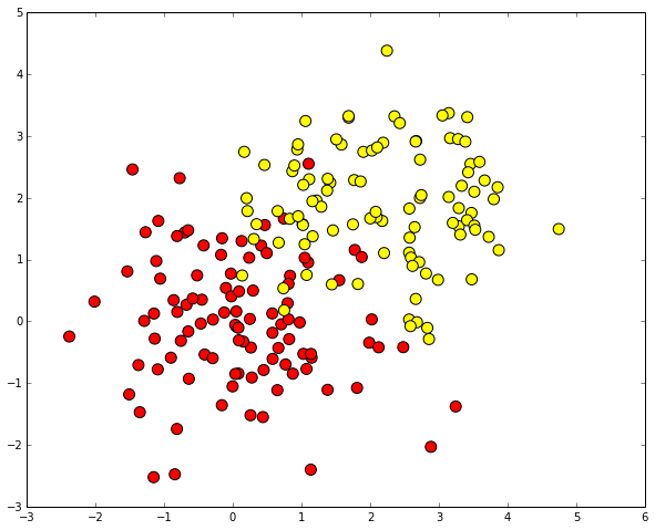
Let's try to separate these two classes, having trained a decision tree. Visualize the resulting class separation boundary.
from sklearn.tree import DecisionTreeClassifier # min_samples_leaf , # clf = DecisionTreeClassifier(min_samples_leaf=5) clf.fit(train_data, train_labels) xx, yy = get_grid(train_data) predicted = clf.predict(np.c_[xx.ravel(), yy.ravel()]).reshape(xx.shape) plt.pcolormesh(xx, yy, predicted, cmap='autumn') plt.scatter(train_data[:, 0], train_data[:, 1], c=train_labels, s=100, cmap='autumn') 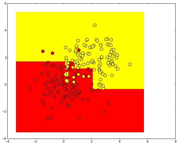
We carry out the same procedure, but now we predict the real probabilities of belonging to the first class.
Strictly speaking, these are not probabilities, but normalized numbers of objects of different classes from one leaf of the tree.
For example, if there are 5 positive objects (labeled 1) and 2 negative (labeled 0) in a sheet,
then, instead of predicting label 1 for all objects that fall on this sheet, it will be predicted
the value of 5/7.
predicted_proba = clf.predict_proba(np.c_[xx.ravel(), yy.ravel()])[:, 1].reshape(xx.shape) plt.pcolormesh(xx, yy, predicted_proba, cmap='autumn') plt.scatter(train_data[:, 0], train_data[:, 1], c=train_labels, s=100, cmap='autumn') 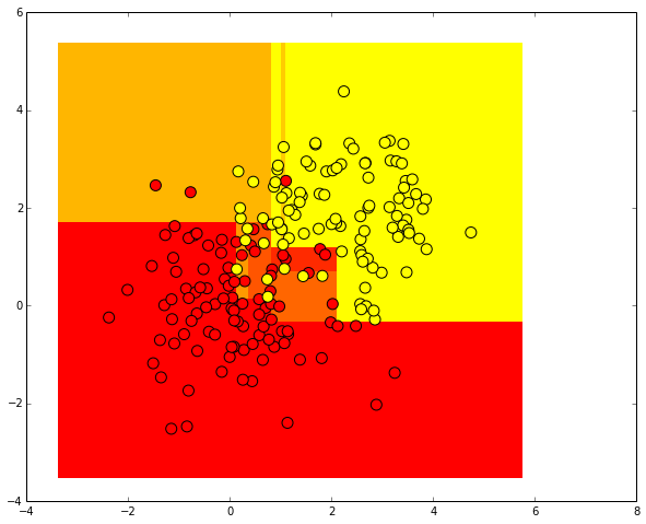
Generate randomly distributed test data.
test_data = np.random.normal(size=(100, 2), loc = 1) predicted = clf.predict(test_data) Display them. Since the labels of test objects are unknown, we draw them in gray.
plt.scatter(test_data[:, 0], test_data[:, 1], c="gray", s=100) 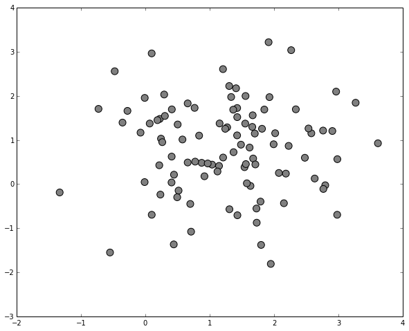
Let's see how the decision tree classified test cases. For contrast, use a different color range.
plt.pcolormesh(xx, yy, predicted_proba, cmap='autumn') plt.scatter(train_data[:, 0], train_data[:, 1], c=train_labels, s=100, cmap='autumn') plt.scatter(test_data[:, 0], test_data[:, 1], c=predicted, s=100, cmap='cool') 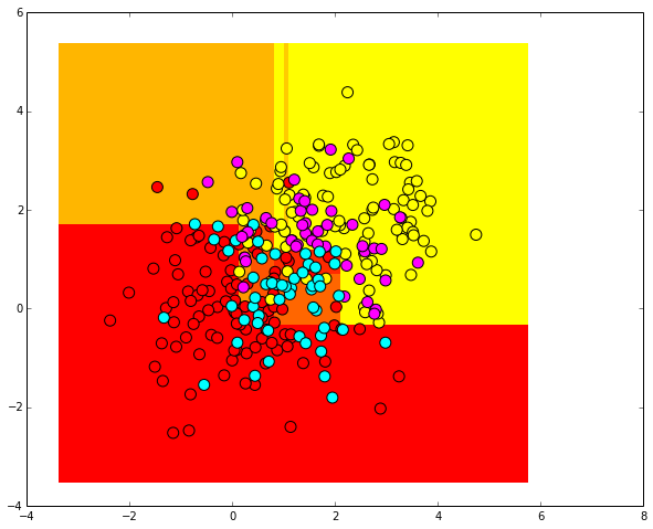
Pros and cons of approach
Here we got acquainted with the simplest and most intuitive classification method, the decision tree, and looked at how it is used in the Scikit-learn library in the classification task. So far we have not discussed how to assess the quality of classification and how to deal with retraining decision trees. Note the pros and cons of this approach.
Pros:
- Generation of clear classification rules that are understandable to a person, for example, “if age is <25 and interest in motorcycles, refuse credit”
- Decision trees can be easily visualized.
- Relatively fast learning and classification processes
- Small number of model parameters
- Support for both numeric and categorical features
Minuses:
- The separating boundary built by the decision tree has its limitations (consists of hypercubes), and in practice the decision tree in terms of the quality of classification is inferior to some other methods
- The need to cut off the branches of the tree (pruning) or set the minimum number of elements in the leaves of the tree or the maximum depth of the tree to combat retraining. However, retraining is the problem of all machine learning methods.
- Instability. Small changes in data can significantly change the constructed decision tree. They are struggling with this problem with the help of decision tree ensembles
- The problem of finding the optimal decision tree is NP-complete; therefore, in practice, heuristics are used such as a greedy search for a feature with maximum information gain, which do not guarantee finding a globally optimal tree
- Difficult supported gaps in the data. Friedman estimated that it took 50% of the CART code to support data gaps.
Part 3. An example of one of the tricks that we teach
Let us take a closer look at one of the tricks actually used by many participants in Kaggle competitions, in this case Stanislav Semenov (4th place in the current Kaggle world ranking at the time of writing) in solving the problem “Greek Media Monitoring Multilabel Classification (WISE 2014)”. The task was to classify articles on topics. The organizers of the competition shared a training sample of about 65 thousand articles submitted with the help of bag models of words and TF-IDF in the form of vectors of length ~ 300 thousand. For each document, it was indicated which topics it can be attributed to (from one topic to thirteen different, on average, one or two). It was necessary to predict which topics include ~ 35 thousand articles from the test sample.
We divide the training sample into validation (validation) and left (holdout) parts in a ratio of 80:20. The test sample will be split again into two parts. On one we will train the linear machine of support vectors ( LinearSVC in Scikit-learn), with the help of the second we will select the parameter C, so as to maximize the measure of the quality of classification F1 - the target one in this competition. The holdout sample remains at the very end, the model is checked on it before sending the solution. This is a common practice that allows you to combat retraining in the process of cross-validation.
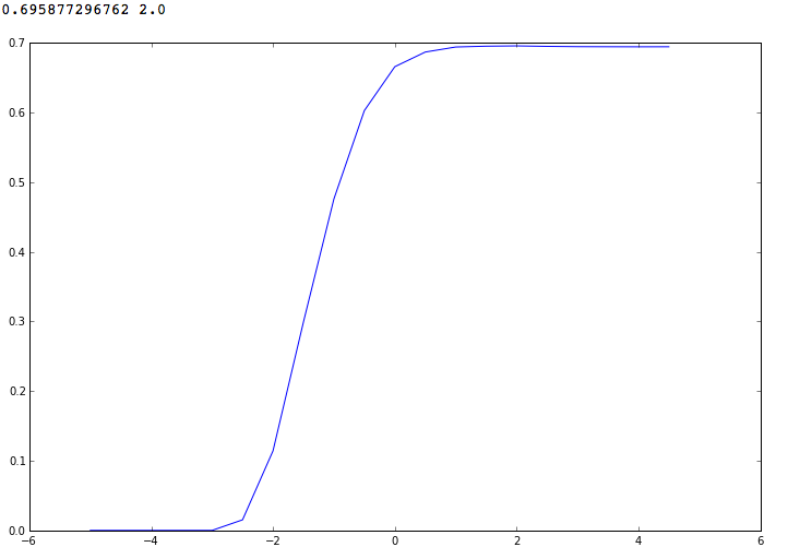
When iterating through a parameter in the range from 10 ^ -5 to 10 ^ 5, we get the following picture. The maximum value of the F1-measure is obtained at C = 100 (10 ^ 2) and is equal to ~ 0.6958.
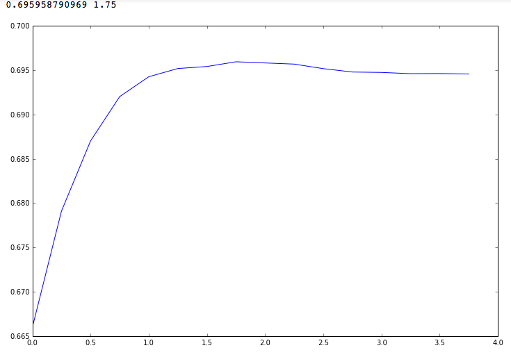
Let's look through the parameters in a narrower range - from 10 ^ 0 to 10 ^ 4. We see that F1 does not tend asymptotically to 0.7 with increasing parameter C, as it may seem, but has a local maximum at C = 10 ^ 1.75
If you send a solution obtained on a test sample using LinearSVC with the parameter C = 10 ^ 1.75, the F1 metric is 0.61, which is quite far from the best assumptions.
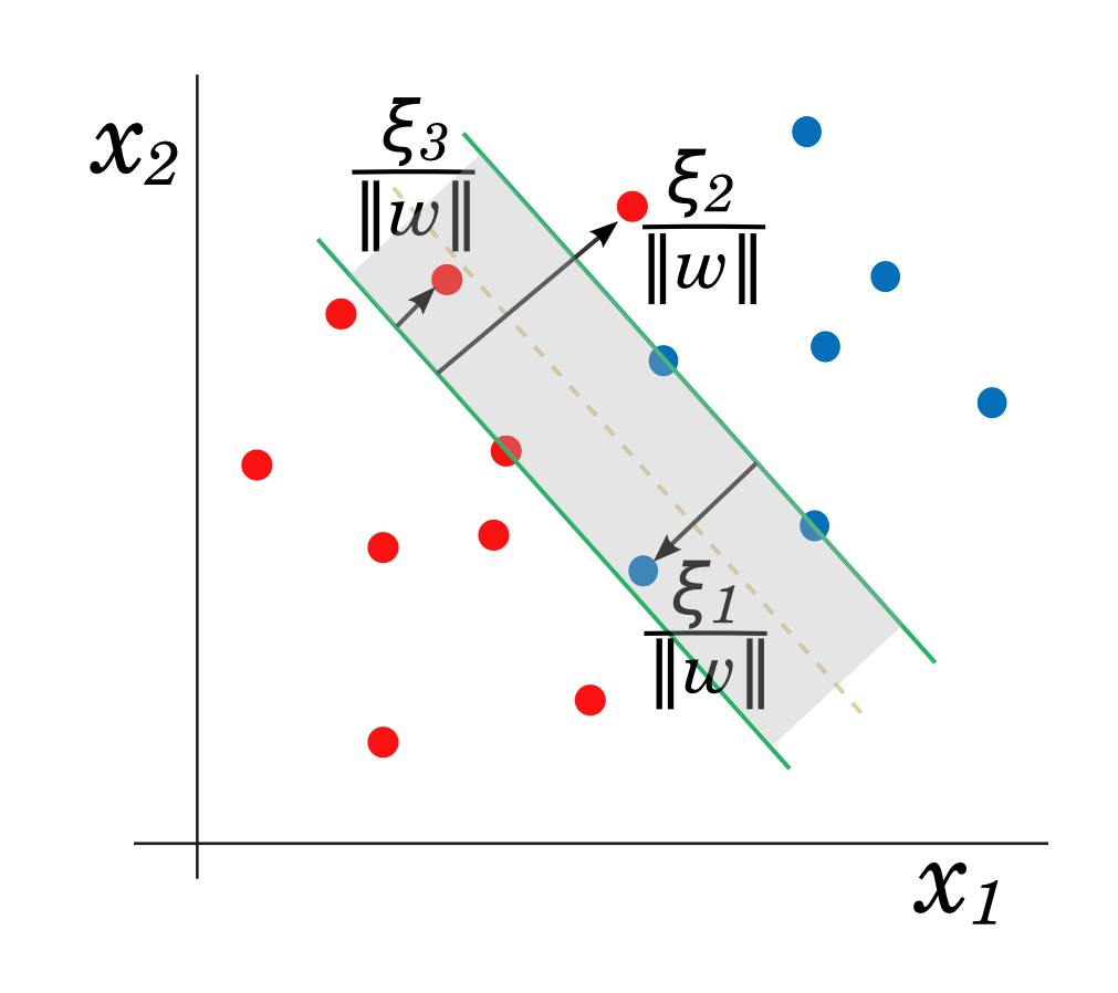
But let's think about how SVM classifies objects in the simplest case of binary classification. In this case, whether the document is related to a topic or not. For each object, the distance from it to the constructed separating hyperplane is considered.
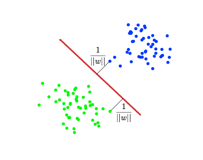
If this distance is positive, the object belongs to one class, otherwise - to another. It turns out that the boundary value of the distance to the separating hyperplane is equal to 0. But who said that this value is optimal for classification? Indeed, in the more complicated case of linear inseparability, the picture may not be so simple, and the hyperplane that separates the classes will not be absolutely unmistakable. In this case, the optimal (to maximize the F1 classification measure) threshold for the distance to the hyperplane may differ from 0.
In Scikit-learn, the distance from objects to the border constructed by the LinearSVC algorithm can be obtained using the decision_function method of the LinearSVC class.
Let us see how the quality of classification (F1) will change if we change the threshold of the distance from the object to the separating hyperplane. For example, in the case of a threshold equal to 0.1, objects that are one side more than 0.1 from the hyperplane will be classified positively, and the rest - negatively.
When the threshold changes from -2 to 2, training LinearSVC on one part of the test sample (80%) and tracking the F1-measure on the other part (20%), we get the following picture.

It turns out that to maximize the F1-measure it is better to use the cut-off threshold for the distance to the hyperplane equal to -0.5.
In this case, the F1-measure on the test sample reaches 0.763, and if you train the algorithm on the entire training sample and use the threshold of -0.5 to classify on the test sample, you can reach F1 = 0.73 for the public sample, which immediately “raises” the top 5% the rating of this Kaggle competition (at the time of writing).
Part 4. Some useful GitHub repositories for programming and machine learning
This is far from an exhaustive list of cool GitHub repositories for programming, data analysis and machine learning in Python. Almost all of them are IPython notebook sets. Some of the materials in my course described above are a translation of these.
- The course of programming in the Python language, the basis of the site introtopython.org .
- "Data science IPython notebooks" - a lot of quality notebooks for the main Python libraries for data analysis - NumPy, SciPy, Pandas, Matplotlib, Scikit-learn. Apache Spark and Kaggle Titanic: Machine Learning from Disaster.
- Harvard Data Analysis Course
- "Interactive coding challenges" - a selection of basic tasks on data structures, graphs, sorting, recursion and more. For many tasks, solutions and explanatory material with pictures are given.
- Olivier Griselle repository (one of the authors of the Scikit-learn library) with IPython training notebooks . One more .
- Scikit -learn tutorial, also from authors
- Analysis of the tasks of the course Andrew Ng "Machine learning" in Python
- Materials in addition to the book "Mining the Social Web (2nd Edition)" (Matthew A. Russell, O'Reilly Media)
- Tutorial on the use of ensembles to solve problems Kaggle.
- The XGBoost library , which is used by most Kaggle competition winners. You can also get acquainted with their success stories. XGBoost is good in prediction quality, effectively implemented, well paralleled.
- Data Collection FiveThirtyEight. Just a bunch of interesting datasets.
- Forecasting US election results. A good example of analyzing data with Pandas
I hope these materials will help you in learning / teaching Python and analyzing data.
The list of cool repositories with IPython notebooks (and simply with Python code), of course, can be continued. For example, in the comments.
Source: https://habr.com/ru/post/270449/
All Articles