How I won the Beeline BigData Contest

Everyone has already heard about machine learning from Beeline many times and even read articles ( one , two ). Now the competition is over, and so it happened that the first place went to me. And although only hundredths of a percent were separated from the previous participants, I would still like to tell you what I did. In fact - nothing incredible.

Data preparation

It is said that 80% of the time data analysts spend on the preparation of data and preliminary modifications and only 20% of them are directly analyzed. And it is not so casual, as “garbage in - garbage out”. The process of preparing the initial data can be divided into several stages, which I propose to go through.

Emission correction

After a careful study of the histograms, it becomes clear that quite a lot of outliers have crept into the data. For example, if you see that 99.9% of observations of variable X are concentrated on the [0; 1] segment, and 0.01% of observations throws out over a hundred, then it is quite logical to do two things: first, introduce a new column to indicate strange events, and second, replace emissions with something sensible.
')

data["x8_strange"] = (data["x8"] < -3.0)*1 data.loc[data["x8"] < -3.0 , "x8"] = -3.0 data["x31_strange"] = (data["x31"] < 0.0)*1.0 data.loc[data["x31"] < 0.0, "x31"] = 0.0 data["x40_zero"] = (data["x40"] == 0.0)*1.0 

Normalization of distributions

In general, working with normal distributions is extremely pleasant, since many statistical tests are tied to the hypothesis of normality. Modern methods of machine learning, this applies to a lesser extent, but still bring the data to a reasonable mind is important. Especially important for methods that work with distances between points (almost all clustering algorithms, k-neighbors classifier). In this part of the data preparation, I managed the standard approach: I log everything that is distributed more densely around zero. Thus, for each variable, I selected a transformation that gave a more pleasant look. Well, after that I scaled everything into a segment [0; 1]

Text variables

In general, text variables are a storehouse for data mining, but in the source data there were only hashes, and the names of the variables were anonymized. Therefore, only the standard routine: replace all rare hashes with the word Rare (rare = less common 0.5%), replace all missing data with the word Missing and deploy as a binary variable (since many methods, including xgboost, are not able to categorical variables) .

 data = pd.get_dummies(data, columns=["x2", "x3", "x4", "x11", "x15"]) for col in data.columns[data.dtypes == "object"]: data.loc[data[col].isnull(), col] = 'Missing' thr = 0.005 for col in data.columns[data.dtypes == "object"]: d = dict(data[col].value_counts(dropna=False)/len(data)) data[col] = data[col].apply(lambda x: 'Rare' if d[x] <= thr else x) d = dict(data['x0'].value_counts(dropna=False)/len(data)) data = pd.get_dummies(data, columns=data.columns[data.dtypes == "object"]) 

Feature engineering

This is what we all love data science for. But everything is encrypted, so this item will have to be omitted. Nearly. After scrutinizing the graphs, I noticed that x55 + x56 + x57 + x58 + x59 + x60 = 1, which means that these are some shares. Let's say what percentage of money a subscriber spends on SMS, calls, the Internet, etc. This means that of particular interest are those comrades who have any of the shares of more than 90% or less than 5%. Thus we get 12 new variables.

 thr_top = 0.9 thr_bottom = 0.05 for col in ["x55", "x56", "x57", "x58", "x59", "x60"]: data["mostly_"+col] = (data[col] >= thr_top)*1 data["no_"+col] = (data[col] <= thr_bottom)*1 

Remove NA

Everything is very simple here: after all distributions are brought to a reasonable form, you can safely replace NA-patches with the mean or median (now they almost coincide). I tried to remove from the training sample those lines where more than 60% of the variables are NA, but this did not end well.

Regression as a regressor

The next step is not so banal. From the distribution of classes, I assumed that age groups are ordered, that is, 0 <1 ... <6 or vice versa. And if so, then you can not classify, and build a regression. It will work poorly, but its result can be transferred to other algorithms for learning. Therefore, we start the usual linear regression with the loss function huber and optimize it through a stochastic gradient descent.

 from sklearn.linear_model import SGDRegressor sgd = SGDRegressor(loss='huber', n_iter=100) sgd.fit(train, target) test = np.hstack((test, sgd.predict(test)[None].T)) train = np.hstack((train, sgd.predict(train)[None].T)) 

Clustering

The second interesting thought I tried: k-means data clustering. If there is a real structure in the data (and it should be in the subscriber data), then k-means will feel it. At first I took k = 7, then added 3 and 15 (twice as much and twice as less). The predictions of each of these algorithms are the cluster numbers for each sample. Since these numbers are not ordered, it is impossible to leave them with numbers, it is necessary to be binarized. Total + 25 new variables.

 from sklearn.cluster import KMeans k15 = KMeans(n_clusters=15, precompute_distances = True, n_jobs=-1) k15.fit(train) k7 = KMeans(n_clusters=7, precompute_distances = True, n_jobs=-1) k7.fit(train) k3 = KMeans(n_clusters=3, precompute_distances = True, n_jobs=-1) k3.fit(train) test = np.hstack((test, k15.predict(test)[None].T, k7.predict(test)[None].T, k3.predict(test)[None].T)) train = np.hstack((train, k15.predict(train)[None].T, k7.predict(train)[None].T, k3.predict(train)[None].T)) 

Training

When the data preparation was completed, the question arose which machine learning method to choose. In principle, the answer to this question has long been known .

In fact, besides xgboost I tried the k-neighbors method. Despite the fact that in spaces of high dimension it is considered ineffective, I managed to achieve 75% (a small step for a person and a big step for k-neighbors), considering the distance not in the usual Euclidean space (where the variables are equal), and correcting for the importance variables as shown in the presentation .

However, all these are toys, and really good results were not yielded by a neural network, not a logistic regression and not k-neighbors, but what was expected - xgboost. Later, when I came to Beeline’s defense, I learned that they also achieved better results with the help of this library. For classification tasks, it is already something of the “gold standard” type.

"When in doubt - use xgboost"
Owen Zhang , top-2 on Kaggle.

Before starting to really start up really and get excellent results, I decided to see how really important are all the columns that were given, and those that I created by expanding the hashes and clustering using the K-Means method. To do this, I made a light boost (not very many trees), and built columns sorted by importance (according to xgboost).

 gbm = xgb.XGBClassifier(silent=False, nthread=4, max_depth=10, n_estimators=800, subsample=0.5, learning_rate=0.03, seed=1337) gbm.fit(train, target) bst = gbm.booster() imps = bst.get_fscore()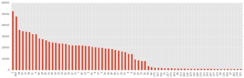 

My opinion is that those columns, the importance of which is rated as “insignificant” (a diagram is constructed only for the most important 70 variables out of 335), contain more noise than actually useful correlations, and learning from them is to harm yourself ( ie retrain ).

It is also interesting to note that the first important variable is x8, and the second is the results of the SGD regression added by me. Those who tried to participate in this competition, probably puzzled that for the variable x8, if it separates the classes so well. On protection in Beeline, I could not resist and did not ask what it was. It was AGE! As I explained, the age specified in the purchase of the tariff, and the age obtained in the polls do not always match, so yes, the participants did determine the age group, including by age.



Through short-lived experiments, I realized that leaving 120 columns is better than leaving 70 or leaving 170 (in the first case, apparently, something useful is still being thrown away, in the second, the data is contaminated by something useless).
Now it was necessary to push. The two xgboost.XGBClassifier parameters that deserve the most attention are eta (aka learning rate) and n_estimators (number of trees). The remaining parameters did not change the results very much (therefore, I set max_depth = 8, subsample = 0.5, and the rest parameters by default).

There is a natural relationship between the optimal values ​​of eta and n_estimators - the lower the eta (learning rate), the more trees are needed to achieve maximum accuracy. And here we are really confronted with the optimum, after which the addition of additional trees causes only retraining, worsening the accuracy of the test sample. For example, for eta = 0.02, approximately 800 trees will be optimal:



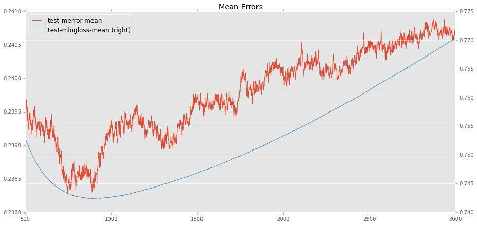
At first I tried working with average eta (0.01-0.03) and saw that depending on the random state (seed) there is a noticeable variation (for example, for 0.02 the score varies from 76.7 to 77.1), and also noticed that this variation becomes smaller with decreasing eta. It became clear that large eta are not suitable in principle (how can a model be so good, so dependent on the seed?).

Then I chose the eta, which I can afford on my computer (I would not like to consider days). This is eta = 0.006. Next, it was necessary to find the optimal number of trees. In the same way as shown above, I found that 3400 trees would be suitable for eta = 0.006. Just in case, I tried two different seed (it was important to understand whether the fluctuations are large).

 for seed in [202, 203]: gbm = xgb.XGBClassifier(silent=False, nthread=10, max_depth=8, n_estimators=3400, subsample=0.5, learning_rate=0.006, seed=seed) gbm.fit(trainclean, target) p = gbm.predict(testclean) filename = ("subs/sol3400x{1}x0006.csv".format(seed)) pd.DataFrame({'ID' : test_id, 'y': p}).to_csv(filename, index=False) 

Each ensemble on the usual core i7 was counted for an hour and a half. It is an acceptable time when the competition takes one and a half months Fluctuations on the public leaderboard were small (for seed = 202 received 77.23%, for seed = 203 77.17%). I sent the best of them, although it is very likely that another would be just as good on a private leaderboard. However, we will not know.

Now a little about the contest itself. The first thing that catches the eye of someone familiar with Kaggle is the slightly unusual rules of submission. At Kaggle, the number of sambiches is limited (depending on the competition, but as a rule, not more than 5 per day), here it’s also sub-unlimited, which allowed some participants to send results as much as 600 times. In addition, the final submission had to choose one, and on Kaggle it is usually allowed to choose any two, and the account on the private leaderboard is considered the best of them.

Another unusual thing is anonymized columns. On the one hand, it practically deprives any opportunity for feature design. On the other hand, this is partly understandable: columns with real names would give a powerful advantage to people versed in mobile communications, and the purpose of the competition was clearly not the case.