Solving the problem of credit scoring in the studio Microsoft Azure Machine Learning
Summary
Predict whether a customer pays a loan or not. The challenge was proposed on an online tournament hosted by one bank. One example of its solution can be found here . Our goal is to build a solution on the Microsoft Azure platform.
Formulation of the problem
The bank requests the applicant's credit history at the three largest Russian credit bureaus. We are provided with a sample of Bank clients in the SAMPLE_CUSTOMERS (CSV) file. The sample is divided into parts “train” and “test”. From the “train” sample, we know the value of the target variable bad - the presence of a “default” (the client assumes a delay of 90 or more days during the first year of using the loan).
The SAMPLE_ACCOUNTS (CSV) file contains data from the responses of credit bureaus to all inquiries on relevant clients. The format of the data from the response of the bureau is information about the accounts of a person transmitted by other banks to the bureau. The data format is described in detail in the ACCOUNT_DATA_FORMAT file.
On the “train” sample, it is necessary to build a model that determines the probability of a “default”, and put down the probabilities of “default” for clients from the “test” sample.
')
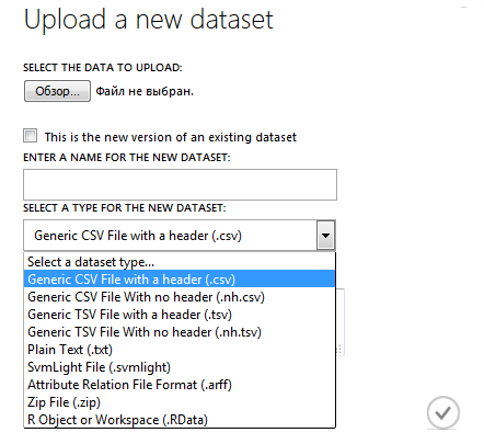
Import dataset into studio
The original data are in CSV format, but the studio correctly recognizes CSV with comma-delimited only. Save the source files with customer information SAMPLE_ACCOUNTS.CSV and SAMPLE_CUSTOMERS.CSV with the required delimiters (for short, SAMPLE_ACCOUNTS.csv was saved as Sdvch.csv) and load them into azure.
Primary processing
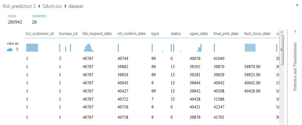
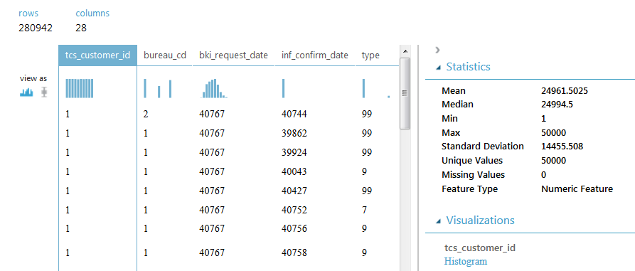
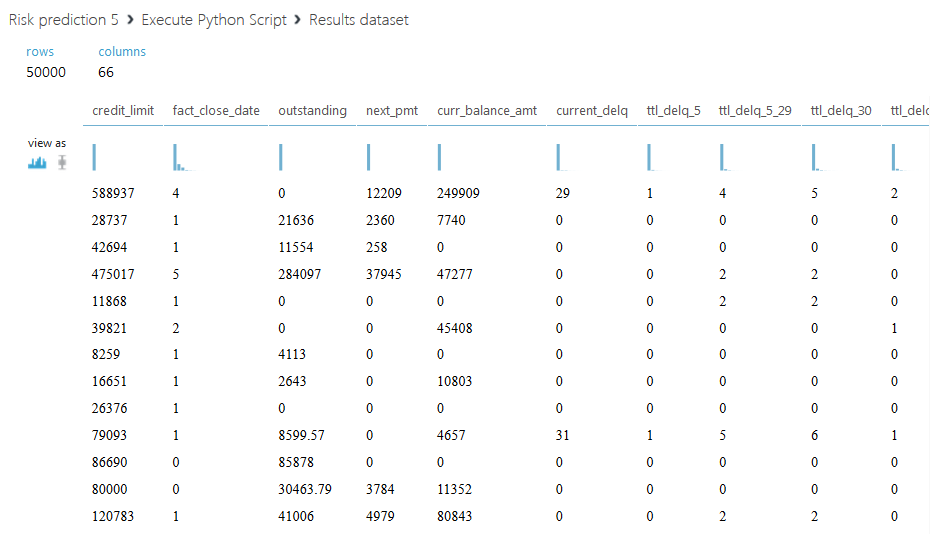
SAMPLE_ACCOUNTS contains 280942 rows and 28 columns, each row contains information on one loan. The column with customer IDs contains 50,000 unique values, which means there can be several lines for each customer. Note that some loans are repeated, and the values of some fields are missing. The contents of the columns will be revealed further in the course of solving the problem.
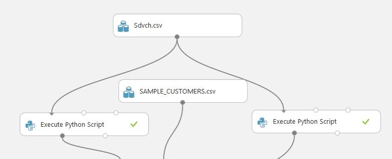
In order to solve the problem, we will consolidate all the information for each client in one line. To do this, run the scripts on Python above the database.
The first script, in fact, consists of the ideas of the solution , which was discussed earlier. Briefly tell them.
Step 1. Drop the duplicate credits (lines) from the data set, leaving the line with the latest information. To do this, we define a set of pillars that will act as a key, these are: tcs_customer_id, open_date, final_pmt_date, credit_limit, currency (id, credit opening date, estimated last payment date, credit limit, currency); column inf_confirm_date (date of confirmation of information on the loan) will determine which of the duplicates remains.
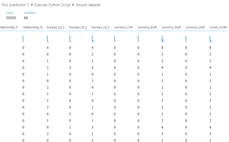
Step 2. Process the columns: pmt_string_84m (timeliness of payments), pmt_freq (payment frequency code), type (agreement type code), status (agreement status), relationship (type of relationship to the agreement), bureau_cd (code of the bureau from which the invoice was received) . We calculate the number of each unique value for each customer and write these values in new columns.
Step 3. Convert the fact_close_date field, which contains the date of the last actual payment, so that it contains only 2 values: 0 - there was no last payment, 1 - the last payment was.
Step 4. We will translate all credit limits to rubles. For simplicity, the course is taken in 2013.
Step 5. Fill in the gaps in the data 0 and perform the final grouping (with summation) by client, with the columns bki_request_date, inf_confirm_date, pmt_string_start, interest_rate, open_date, final_pmt_date, inf_confirm_date_max. These are the dates and the interest paid on the loan.
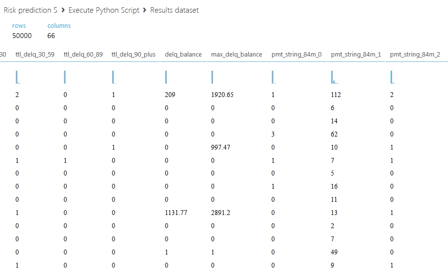
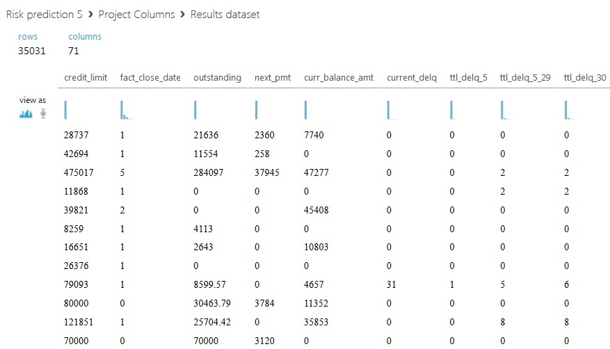
Below is the resulting dataset.
Let us dwell on the second script. We propose not only to sum up all credit limits for each client, but to divide the entire amount into two parts: the active credit limit, with a status value of 00, and a closed one - with all other statuses. We also introduce another column with the ratio of the total active limit to - closed, if the sum of the closed limit is zero, then the field will be filled with the letter A. The code of the second script is shown below.
def azureml_main(dataframe1): from pandas import read_csv, DataFrame,Series import numpy SampleAccounts=dataframe1 SampleAccounts.final_pmt_date[SampleAccounts.final_pmt_date.isnull()] = SampleAccounts.fact_close_date[SampleAccounts.final_pmt_date.isnull()].astype(float) SampleAccounts.final_pmt_date.fillna(0, inplace=True) # sumtbl = SampleAccounts.pivot_table(['inf_confirm_date'], ['tcs_customer_id','open_date','final_pmt_date','credit_limit','currency'], aggfunc='max') #sumtbl - SampleAccounts = SampleAccounts.merge(sumtbl, 'left', left_on=['tcs_customer_id','open_date','final_pmt_date','credit_limit','currency'], right_index=True, suffixes=('', '_max')) # SampleAccounts=SampleAccounts.drop_duplicates(['tcs_customer_id','open_date','final_pmt_date','credit_limit','currency']).reset_index() df1=SampleAccounts.drop('index',axis=1) curs = DataFrame([33.13,44.99,36.49,1], index=['USD','EUR','GHF','RUB'], columns=['crs']) df2 = df1.merge(curs, 'left', left_on='currency', right_index=True) df2.credit_limit = df2.credit_limit * df2.crs # df2=df2.drop(['crs'], axis=1) # df3 = df2[['tcs_customer_id','credit_limit','status']] df3['act_lim']=df3.credit_limit[df3.status==0] df3.act_lim.fillna(0, inplace=True) df4=df3.copy() df4['credit_limit'] = numpy.where(df3['status']==0, 0, df3.credit_limit) df5=df4.groupby('tcs_customer_id').sum() df5.rename(columns={'credit_limit':'closed_limit'}, inplace=True) df6=df5.drop('status',axis=1) df6['otn_lim']=numpy.where(df6.closed_limit==0, 'A', df6.act_lim/df6.closed_limit) return df6 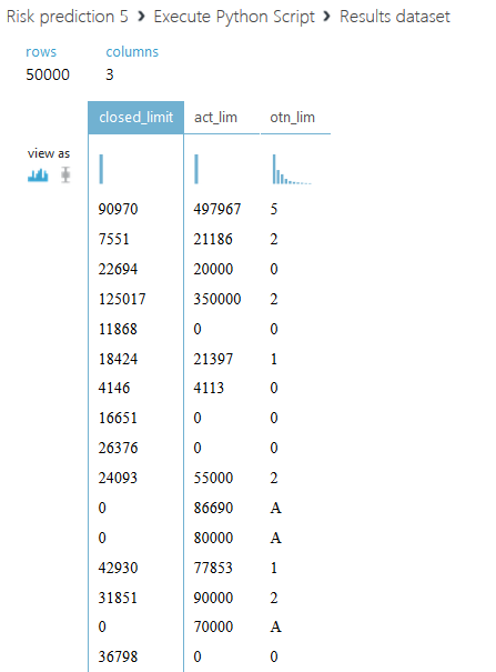
Azure processing
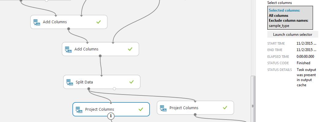
Using two “Add Columns” blocks, we connect the bases of the resulting scripts processing with the SAMPLE_CUSTOMERS file.


Next, divide the sample into two parts using the “Split Data” block. Choose a regular expression mode and set a condition on the column “sample_type”, we need lines with the value “train”.
Using the “Project Columns” block, we select the columns remaining for processing. We will compare two data sets: on the left with all received columns (except sample_type, it is the same “train” everywhere), on the right without our modification, that is, with the exception of the active and closed limit columns and their relationship (and sample_type).
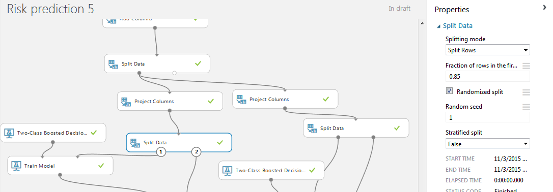
Now add to the project another pair of modules "Split Data". This time we use a pseudo-random row separation into two parts with a given “random seed” field. This is necessary so that the division of the sample into two parts takes place equally for the left and right bases. The percentage for training and testing is 85% and 15%. This is explained by the fact that in our case the base with 50,000 clients has already been divided into two train and test samples. In theory, we would have to train 100% of the base train and put the result in test, but since we are learning and testing on the train, the ratio was chosen more favorable than the usual 75/25 or 80/20.
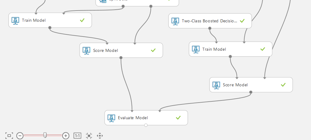
To train the model, we will use a two-class elevated decision tree (two-class boosting) with standard values. We also add the modules Train Model and Score Model. In the “Train Model” we indicate the required column for predicting bad.
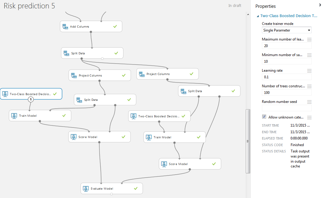
Visualization of the left block “Score Model”.

It remains to connect the outputs of the Score Model modules with the inputs of the Evaluate Model block, which allows you to compare the results of the two methods. In our case - the results of the work of one classification method for two different data sets.
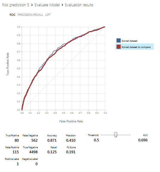
The following screen shows the visualization of the Evaluate Model block, that is, the prediction results. The blue line corresponds to the left database (with all received columns), the red line to the right one (with the exception of active, closed limit columns and their ratio).

Conclusion
Given the distribution of seats held tournament
- AUC 0.7057
- AUC 0.7017
- AUC 0.7012
- AUC 0.6997
Thanks for attention!
Resources used
Source: https://habr.com/ru/post/270201/
All Articles