Kaggle competition for analyzing population survey data
The kaggle is currently hosting the USA Census 2013 competition for finding interesting facts in the American Community Survey. The data of this survey are available in free access, details can be found here .
Kaggle chose to analyze two areas - personal information (gender, age, marital status, etc.) and information about households (various characteristics of housing, household income, tax payments, etc.). I want to share my results , which are focused on the differences of households depending on the type of ownership of their housing - ownership with restrictions (mortgage or loan), ownership without restrictions and not owning (renting).
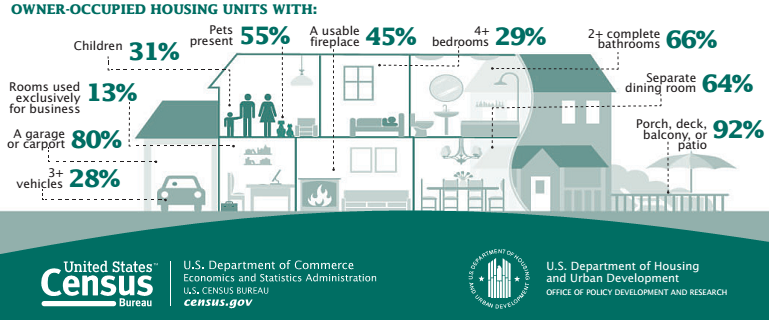
infographics: American Housing Survey Factsheets
The American Community Survey (ACS) data is weighted, the study design is given by repeated weights. Therefore, all statistics, where it makes sense, are weighted. All households in the country are divided into 2351 clusters on a geographical basis with a population of about 100 thousand people in each cluster. These clusters are called PUMAs (public use microdata areas). Next, we look at the target audience everywhere, in which households either own housing with restrictions on property, or own their housing, or rent housing. This target audience is about 86% of the total number of households in the country.
Comparing Mortgage and Rental Costs
The following two graphs show the average household spending on mortgages and rent in these clusters. The units of measurement of the first graph are the share of the mortgage / rent costs of household income, the second graph shows the household costs of mortgage / rent in dollars per month. The red line on both graphs shows the median values for renting a relatively small mortgage interval.
')

It can be seen that, on average, the share of housing costs of households that rent it is higher than that of households that purchased housing as a mortgage. But in absolute figures, the picture changes to the opposite - the monthly payments on average are larger for the second group. These observations are valid for almost all regions.
Prevailing type of ownership of housing depending on the level of household income
Consider the distribution of shares of households with one of the three types of property rights by the deciles of their income per year. That is, we divide the target audience into 10 equal parts (taking into account weights) according to their income level. The first group includes 10% of households with the lowest income, and so on, by increasing the level of household income.
We get the following result (the red is the share of those who rent housing, light gray is the share of owners without any restrictions, blue is the share of mortgage owners)

It is easy to see the trend of differences in shares of those who rent housing and owners with unfinished mortgage payments, depending on the level of income. Approximate equality of these shares (37-38%) is achieved in 5 deciles. The share of owners without burden on housing, starting from 3 deciles, with an increase in the level of income drops ~ 1.5% per decile, except for the last group with the highest incomes.
The impact of social factors on the type of ownership of housing
Consider three types of families.
Previously, we divided the entire target audience into deciles by household income per year. Consider the distribution of income levels of each of these classes of families along the obtained boundaries of the found deciles.
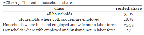
As expected, the income of the family in which both spouses work has a significant shift towards upper deciles. Based on previous information, it can be assumed that the proportion of families of this class who rent housing is less than the average figures throughout the country. So it is, less than almost twice

As we see, families in which only the wife works, and the husband does not work and does not look for work, are less wealthy compared to families where both spouses work. Is it true that the share of families who rent housing in a class where only the wife works is more than the share of tenants in families with both working spouses? It turns out no.
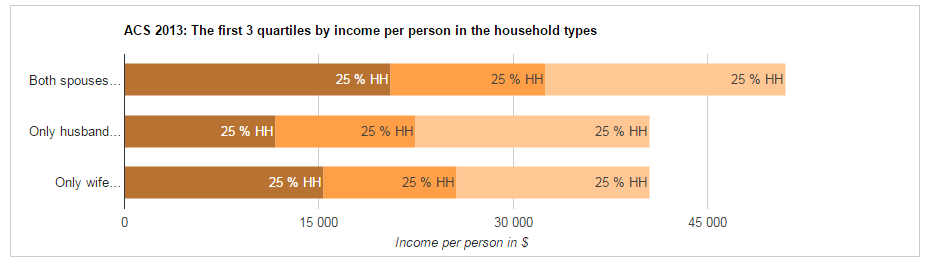
Let us make sure that the average income per person per year, in families in which both spouses work, exceeds that for the other two classes of families. The graph below shows the range of average income per person in the first three apartments.
And now we will look at the distribution of shares of types of ownership in these classes by the quartiles of income of all households.
In each group of the same level of income, families in which only the wife works have the lowest share of tenants. We show that these differences are statistically significant. To do this, set the design of the study. After that we find the logistic regression of the form

We get the following table of model coefficients with standard deviation values and p.value values

That is, in all four cases, the coefficient B_2 is significantly different from 0. For a linear combination of the coefficients B_2 - B_1, using the Wald test, it can be shown that the coefficient B_2 is significantly less than the coefficient B_1 in all four cases.
This proves our assumption that families where only a spouse works are less likely to rent housing than the other two classes of families. It can be shown that the resulting difference goes to the share of families who have their own housing without restricting the right of ownership to it.
Those who are interested can follow this link to kaggle , where full-fledged Google Charts with controls and tooltips are placed, the code for all calculations in the R language and additional information and graphics.
Kaggle chose to analyze two areas - personal information (gender, age, marital status, etc.) and information about households (various characteristics of housing, household income, tax payments, etc.). I want to share my results , which are focused on the differences of households depending on the type of ownership of their housing - ownership with restrictions (mortgage or loan), ownership without restrictions and not owning (renting).
infographics: American Housing Survey Factsheets
The American Community Survey (ACS) data is weighted, the study design is given by repeated weights. Therefore, all statistics, where it makes sense, are weighted. All households in the country are divided into 2351 clusters on a geographical basis with a population of about 100 thousand people in each cluster. These clusters are called PUMAs (public use microdata areas). Next, we look at the target audience everywhere, in which households either own housing with restrictions on property, or own their housing, or rent housing. This target audience is about 86% of the total number of households in the country.
Comparing Mortgage and Rental Costs
The following two graphs show the average household spending on mortgages and rent in these clusters. The units of measurement of the first graph are the share of the mortgage / rent costs of household income, the second graph shows the household costs of mortgage / rent in dollars per month. The red line on both graphs shows the median values for renting a relatively small mortgage interval.
')
It can be seen that, on average, the share of housing costs of households that rent it is higher than that of households that purchased housing as a mortgage. But in absolute figures, the picture changes to the opposite - the monthly payments on average are larger for the second group. These observations are valid for almost all regions.
Prevailing type of ownership of housing depending on the level of household income
Consider the distribution of shares of households with one of the three types of property rights by the deciles of their income per year. That is, we divide the target audience into 10 equal parts (taking into account weights) according to their income level. The first group includes 10% of households with the lowest income, and so on, by increasing the level of household income.
We get the following result (the red is the share of those who rent housing, light gray is the share of owners without any restrictions, blue is the share of mortgage owners)
It is easy to see the trend of differences in shares of those who rent housing and owners with unfinished mortgage payments, depending on the level of income. Approximate equality of these shares (37-38%) is achieved in 5 deciles. The share of owners without burden on housing, starting from 3 deciles, with an increase in the level of income drops ~ 1.5% per decile, except for the last group with the highest incomes.
The impact of social factors on the type of ownership of housing
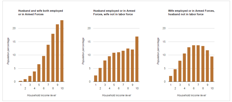
Consider three types of families.
- Both spouses are working or are military personnel
- Only the husband works or is a soldier; the wife does not work and is not looking for work.
- Only the wife works or is a soldier; the husband does not work and is not looking for work.
Previously, we divided the entire target audience into deciles by household income per year. Consider the distribution of income levels of each of these classes of families along the obtained boundaries of the found deciles.
As expected, the income of the family in which both spouses work has a significant shift towards upper deciles. Based on previous information, it can be assumed that the proportion of families of this class who rent housing is less than the average figures throughout the country. So it is, less than almost twice
As we see, families in which only the wife works, and the husband does not work and does not look for work, are less wealthy compared to families where both spouses work. Is it true that the share of families who rent housing in a class where only the wife works is more than the share of tenants in families with both working spouses? It turns out no.
Let us make sure that the average income per person per year, in families in which both spouses work, exceeds that for the other two classes of families. The graph below shows the range of average income per person in the first three apartments.
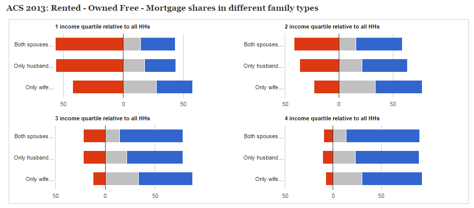
And now we will look at the distribution of shares of types of ownership in these classes by the quartiles of income of all households.
In each group of the same level of income, families in which only the wife works have the lowest share of tenants. We show that these differences are statistically significant. To do this, set the design of the study. After that we find the logistic regression of the form
We get the following table of model coefficients with standard deviation values and p.value values
That is, in all four cases, the coefficient B_2 is significantly different from 0. For a linear combination of the coefficients B_2 - B_1, using the Wald test, it can be shown that the coefficient B_2 is significantly less than the coefficient B_1 in all four cases.
This proves our assumption that families where only a spouse works are less likely to rent housing than the other two classes of families. It can be shown that the resulting difference goes to the share of families who have their own housing without restricting the right of ownership to it.
Those who are interested can follow this link to kaggle , where full-fledged Google Charts with controls and tooltips are placed, the code for all calculations in the R language and additional information and graphics.
Source: https://habr.com/ru/post/270131/
All Articles