How to draw curves graphics in the style of XKCD

Recently I published an article on Habré about a guitar tuner , and many were interested in animated graphics that I used to illustrate sound waves, including the technology for creating such graphs. Therefore, in this article I will share my approach and library on Node.js which will help to build such graphs.

Prehistory

Why make graphics curves?

In general, the idea of ​​creating curves graphs comes from academic culture - not only Russian, but also global.

This approach, when even quite complex scientific information is illustrated by sloppy charts, is a fairly common practice.
')
It is on this nuance that XKCD comics are created, the humor of which is based on simple dependencies interpreted in some unusual manner:



Negligence in the graphs allows you to shift attention from a quantitative assessment to a qualitative one, which in turn contributes to a better perception of new information.

Why write scripts to build graphs?

Firstly, when a publication is prepared where there is a lot of source data or where this data can change during preparation, it is better to compile and store graphs in the form of scripts. In this case, if the data or results change during the preparation of the publication, you can re-arrange the graphs automatically.

Secondly, it is difficult to say how a particular chart will look like in a publication; therefore, it is often necessary to adjust to the size of the fields, indents, and the alignment of the text. This is easiest to do if there is a script and it allows you to rebuild the schedule for a new look by changing the parameters. On the contrary, if the schedule was made without a script in some editor, such manipulations become time consuming.

Thirdly, graphics in the form of scripts are much more convenient to maintain due to the ability to use version control systems - there is always the opportunity to roll back or merge patches without fear of losing working data.

Why Node.js?

There are many libraries for building graphs, including the XKCD effect, there are extensions for matplotlib and a special package for R. However, Javascript has several advantages.

For Javascript, a convenient, convenient browser-based Canvas and Node.js libraries are available that implement this behavior. In turn, the script written for Canvas can be reproduced in the browser, which allows, for example, to display data on the site dynamically. Canvas is also useful for debugging animations in the browser, since drawing actually happens on the fly. Having a drawing script on Node.js, you can use the GIFEncoder package, which makes it very easy to create an animated movie.

Add curvature

The appearance of graphs in the style of XKCD can be obtained by adding random offsets. But these offsets should not be added at every point, otherwise there will simply be a vague schedule, but with some step.



Therefore, any line that needs to be drawn must be broken, and already the nodal points must be shifted by some random variable. Since the incoming line may contain either too small or too large sections, then an algorithm is required that would combine too small into large, and vice versa would break large sections into small ones.

The described behavior can be implemented as follows:

self.replot = function(line, step, radius){ var accuracy = 0.25; if(line.length < 2) return []; var replottedLine = []; var beginning = line[0]; replottedLine.push(beginning); for(var i = 1; i < line.length; i++){ var point = line[i]; var dx = point.x - beginning.x; var dy = point.y - beginning.y; var d = Math.sqrt(dx*dx+dy*dy); if(d < step * (1 - accuracy) && (i + 1 < line.length)){ // too short continue; } if(d > step * (1 + accuracy)){ // too long var n = Math.ceil(d / step); for(var j = 1; j < n; j++){ replottedLine.push({ x: beginning.x + dx * j / n, y: beginning.y + dy * j / n }); } } replottedLine.push(point); beginning = point; }; for(var i = 1; i < replottedLine.length; i++){ var point = replottedLine[i]; replottedLine[i].x = point.x + radius * (self.random() - 0.5); replottedLine[i].y = point.y + radius * (self.random() - 0.5); }; return replottedLine; }; 

The result of such processing:


Since Since random displacements make even the smoothest graphs broken (and the sine wave is the ideal of smoothness), then it is impossible to stop at random displacements — you must return the lost smoothness. One of the ways to return smoothness is to use quadratic curves instead of straight lines.

The quadraticCurveTo method from Canvas represents a drawing with smoothness sufficient for our tasks, but it also requires auxiliary nodes. These nodes can be calculated based on the reference points obtained in the previous step:

  ctx.beginPath(); ctx.moveTo(replottedLine[0].x, replottedLine[0].y); for(var i = 1; i < replottedLine.length - 2; i ++){ var point = replottedLine[i]; var nextPoint = replottedLine[i+1]; var xc = (point.x + nextPoint.x) / 2; var yc = (point.y + nextPoint.y) / 2; ctx.quadraticCurveTo(point.x, point.y, xc, yc); } ctx.quadraticCurveTo(replottedLine[i].x, replottedLine[i].y, replottedLine[i+1].x,replottedLine[i+1].y); ctx.stroke(); 

The resulting smoothed line will correspond exactly to the sloppy shape:

Clumsy Library

Based on the above algorithms, I built a small library. It is based on the Clumsy wrapper class, which implements the desired behavior using the Canvas object.

In the case of Node.js, the initialization process looks like this:

  var Canvas = require('canvas'); var Clumsy = require('clumsy'); var canvas = new Canvas(800, 600); var clumsy = new Clumsy(canvas); 

The main methods of the class are needed to draw the simplest graphics:

  range(xa, xb, ya, yb); //     padding(size); //     draw(line); //   axis(axis, a, b); //   clear(color); //  canvas   tabulate(a, b, step, cb); //      

A more complete list of methods and fields, as well as their description and examples of use can be found in the project documentation for npm .

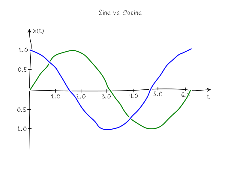
How it works can be demonstrated by the example of sine:

  clumsy.font('24px VoronovFont'); clumsy.padding(100); clumsy.range(0, 7, 2, 2); var sine = clumsy.tabulate(0, 2*Math.PI, 0.01, Math.sin); clumsy.draw(sine); clumsy.axis('x', 0, 7, 0.5); clumsy.axis('y', -2, 2, 0.5); clumsy.fillTextAtCenter("", 400, 50); 

Animation

Getting a moving image on a Canvas in the browser is quite simple, just wrap the rendering algorithm into a function and pass it to setInterval. This approach is useful primarily for debugging, since the result is directly observed. As for the generation of the finished gif on Node.js, in this case, you can use the GIFEncoder library.

For example, take the Archimedes spiral, which we make rotate at a speed of pi radians per second.
When you need to animate a certain graph, it is most convenient to make a separate file that is solely responsible for drawing, and separate files that set animation parameters - fps, movie duration, etc. Let's name the script of the drawing spiral.js and create the Spiral function in it:

  function Spiral(clumsy, phase){ clumsy.clear('white'); clumsy.padding(100); clumsy.range(-2, 2, -2, 2); clumsy.radius = 3; var spiral = clumsy.tabulate(0, 3, 0.01, function(t){ var r = 0.5 * t; return { x: r * Math.cos(2 * Math.PI * t + phase), y: r * Math.sin(2 * Math.PI * t + phase) }; }) clumsy.draw(spiral); clumsy.axis('x', -2, 2, 0.5); clumsy.axis('y', -2, 2, 0.5); clumsy.fillTextAtCenter('', clumsy.canvas.width/2, 50); } //       if(typeof module != 'undefined' && module.exports){ module.exports = Spiral; } 

Then you can view the result in a browser by making a debug page:

  <!DOCUMENT html> <script src="https://rawgit.com/kreshikhin/clumsy/master/clumsy.js"></script> <link rel="stylesheet" type="text/css" href="http://webfonts.ru/import/voronov.css"></link> <canvas id="canvas" width=600 height=600> <script src="spiral.js"></script> <script> var canvas = document.getElementById('canvas'); var clumsy = new Clumsy(canvas); var phase = 0; setInterval(function(){ //  seed  ""  clumsy.seed(123); Spiral(clumsy, phase); phase += Math.PI / 10; }, 50); </script> 

Debugging in the browser is convenient because the result appears immediately. Since no time required to generate frames and compress to GIF format. What may take a few minutes. Saving the page in the .html format and opening in the browser we should see a rotating spiral on the Canvas:



When the graph is debugged, you can use the same spiral.js file to create a script to generate a GIF file:

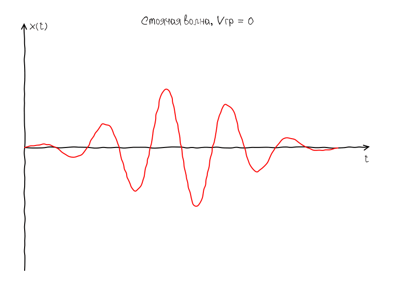
  var Canvas = require('canvas'); var GIFEncoder = require('gifencoder'); var Clumsy = require('clumsy'); var helpers = require('clumsy/helpers'); var Spiral = require('./spiral.js'); var canvas = new Canvas(600, 600); var clumsy = new Clumsy(canvas); var encoder = helpers.prepareEncoder(GIFEncoder, canvas); var phase = 0; var n = 10; encoder.start(); for(var i = 0; i < n; i++){ //  seed  ""  clumsy.seed(123); Spiral(clumsy, phase); phase += 2 * Math.PI / n; encoder.addFrame(clumsy.ctx); }; encoder.finish(); 

In exactly the same way, I created graphics to illustrate the standing wave phenomenon:

Conclusion

So, using such a simple-minded wrapper over a Canvas, you can achieve a rather original drawing of graphs in the style of XKCD. In general, this was the main goal of creating a library.

It is not universal, but if you need to build a fairly simple graph in the style of XKCD, then it copes with this task more than well. Additional features can be implemented independently using the features of HTML5 Canvas.

Full documentation and examples can be found at these links:

github.com/kreshikhin/clumsy

npmjs.com/package/clumsy

The source code is accompanied by a MIT license. Therefore, you can safely use the code sections you are interested in or the entire project code for your own purposes.