Why google voice neural nets search?
Have you ever wondered how voice search works? What magic translates your words into a search query, and almost in real time? Today, we’ll tell you how “Ok, Google!” Has become closer to you by 300 milliseconds and what exactly allows you to talk to your phone in simple human language.

The basis of the current version of Google voice search is an improved algorithm for training neural networks, created specifically for the analysis and recognition of acoustic models. The basis of new, Recurrent Neural Networks ( English: recurrent neural networks - RNN), formed the Neural Network Temporal Classification ( English: Connectionist Temporal Classification - CTC) and discriminant analysis for sequences, adapted for the training of such structures. RNN data is much more accurate, especially in conditions of extraneous noise, and most importantly - they work faster than all previous speech recognition models.
We'll have to start with a little insight into history. For almost 30 years (by the standards of the IT industry, it is an eternity!) Speech recognition was used for speech recognition. “Models of a mixture of (multidimensional) normal distributions” ( eng .: Gaussian Mixture Model - GMM). At first, Google’s voice search also worked with this technology until we developed a new approach to translating sound waves into a meaningful set of characters with which a “classic” text search can operate.
At that time (this happened in 2012) the transfer of Google’s voice search to Deep Neural Networks technology ( Eng .: Deep Neural Networks - DNN) made a real breakthrough in speech recognition. DNNs were better suited for recognizing individual sounds uttered by the user than GMM, making the speech recognition accuracy significantly higher.
In the classical voice recognition system, the recorded audio signal is divided into short (10 ms) fragments, each of which is then analyzed for the frequencies contained in it. The resulting vector of characteristics is driven through an acoustic model (for example, such as DNN), which produces a set of probability distributions among all possible phonemes. The hidden Markov model (often used in pattern recognition algorithms) helps to identify successive structures in this set of probability distributions.
')
After this, the analysis data is combined with other data from alternative sources of information. One of them is the Pronunciation Model ( English: Pronunciation Model), which connects a sequence of sounds into certain words of the intended language. (approx .: Under the "intended" language refers to the language that was selected as the "main" in the voice search settings). Another source is the Language Model: it processes the words obtained and analyzes the whole phrase, trying to assess how likely such a sequence of words is in the target language.
Then all the information goes into the recognition system, which matches all the information to determine the phrase that the user utters. For example, if a user pronounces the word “museum”, then his phonetic record would look like this: / mjuzi @ m /.
It can be difficult to say exactly where the sound / j / ended and / u / began, but in fact it does not matter for the algorithm: the main thing is that all these sounds were uttered.
Our improved acoustic model is based on Recurrent Neural Networks (RNN). Their advantage is that they have feedback loops in their topology, allowing them to simulate temporal dependencies: when the user pronounces / u / in the previous example, his speech machine leaves the pronunciation process of the previous sounds / j / and / m / at the same time. Try to say out loud - «museum». The word comes out instantly, on one exhalation, and the RNN can recognize it.
RNNs are of different types, and for speech recognition we used special RNNs with “long short-term memory” ( English: Long Short-Term Memory - LSTM ). These memory cells and the complicated mechanism of the gates allow the LSTM RNN to memorize information better than other neural networks.
The use of these models alone has already significantly improved the quality of our recognition system, but we did not stop there. The next step was the training of neural networks to recognize phonemes in a phrase without the need to constantly distinguish individual “assumptions” about the probability distribution of each of them.
With the Neural Network Temporal Classification (CTC), the models learned to derive peculiar “peaks”, which represent a sequence of different sounds in the sound wave. They can distinguish different phonemes in the correct sequence of sounds from a language point of view.
The most difficult was the question “How to make the recognition happen in real time?”. After many attempts, we were able to teach streaming unidirectional models to process longer audio intervals than those used in “classical” speech recognition models. While the calculations themselves occur with less frequency. At the same time, the cost of computing resources has actually decreased, and the speed of the recognition system has increased many times over.
In the laboratory, it is easy to recognize speech: in complete silence, you get a high-quality sound track, which you then analyze. Unfortunately, the actual operating conditions of voice search are significantly different from the reference. Someone is talking in the background, cars are passing by, a TV is buzzing somewhere in the distance, a gust of wind flies into the microphone of the smartphone ... All these noises make it difficult for neural networks to process speech, so we taught them to work even in such difficult conditions.
In the process of learning RNN, we mixed artificial noise, reverb, echo, and other typical “pollution” in the daily use of the training samples, which helped to make the recognition system more resistant to background noise.
Now we had a fast and accurate resolver and we were ready to launch it on real voice requests, however, we had to solve another problem.
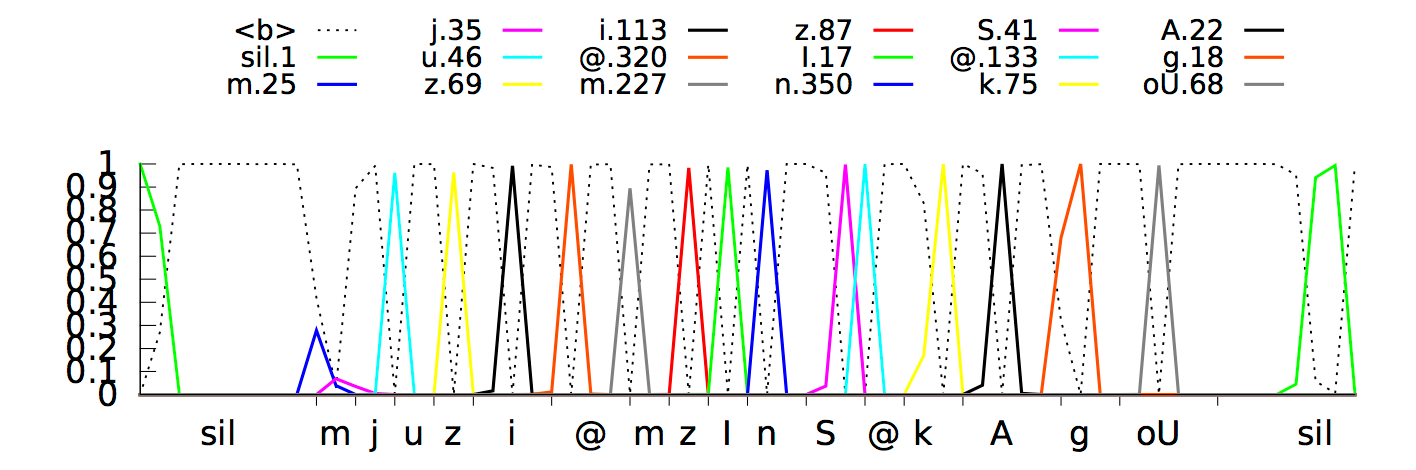
The model predicted phonemes with a delay of about 300 milliseconds, since the neural network "realized" that it would be able to better recognize phonemes by listening to the signal for a little longer. Here is the process of recognition in visual form:
Neural network temporal classification is trying to recognize the phrase "How cold it is outside"
This behavior was logical and worked fine, but it led to slower system responses, which we didn’t want at all. We solved this problem by means of a long training of the neural network to select individual phonemes as close as possible to the “cutoff” of the signal. As a result, speech recognition takes place almost in real time. The current model based on CTC allocates "peaks" of individual phonemes (displayed in different colors) as soon as it identifies them in the incoming audio stream.
The X-axis shows the phonemes defined at each time instant, and the Y-axis shows the posterior probabilities of the distribution of one or another phoneme. The dashed lines mark the variants that the algorithm decided not to single out / recognize as separate sounds.
Now our new algorithm is used in voice control and dictation of the text on your smartphones (so far only on the basis of Android) and the Google application on Android and iOS . It not only uses less computational resources, but more precisely, it works faster, and is still resistant to noise and interference. Try it, hope you enjoy it!
The basis of the current version of Google voice search is an improved algorithm for training neural networks, created specifically for the analysis and recognition of acoustic models. The basis of new, Recurrent Neural Networks ( English: recurrent neural networks - RNN), formed the Neural Network Temporal Classification ( English: Connectionist Temporal Classification - CTC) and discriminant analysis for sequences, adapted for the training of such structures. RNN data is much more accurate, especially in conditions of extraneous noise, and most importantly - they work faster than all previous speech recognition models.
We'll have to start with a little insight into history. For almost 30 years (by the standards of the IT industry, it is an eternity!) Speech recognition was used for speech recognition. “Models of a mixture of (multidimensional) normal distributions” ( eng .: Gaussian Mixture Model - GMM). At first, Google’s voice search also worked with this technology until we developed a new approach to translating sound waves into a meaningful set of characters with which a “classic” text search can operate.
At that time (this happened in 2012) the transfer of Google’s voice search to Deep Neural Networks technology ( Eng .: Deep Neural Networks - DNN) made a real breakthrough in speech recognition. DNNs were better suited for recognizing individual sounds uttered by the user than GMM, making the speech recognition accuracy significantly higher.
As it was before: the work of DNN
In the classical voice recognition system, the recorded audio signal is divided into short (10 ms) fragments, each of which is then analyzed for the frequencies contained in it. The resulting vector of characteristics is driven through an acoustic model (for example, such as DNN), which produces a set of probability distributions among all possible phonemes. The hidden Markov model (often used in pattern recognition algorithms) helps to identify successive structures in this set of probability distributions.
')
After this, the analysis data is combined with other data from alternative sources of information. One of them is the Pronunciation Model ( English: Pronunciation Model), which connects a sequence of sounds into certain words of the intended language. (approx .: Under the "intended" language refers to the language that was selected as the "main" in the voice search settings). Another source is the Language Model: it processes the words obtained and analyzes the whole phrase, trying to assess how likely such a sequence of words is in the target language.
Then all the information goes into the recognition system, which matches all the information to determine the phrase that the user utters. For example, if a user pronounces the word “museum”, then his phonetic record would look like this: / mjuzi @ m /.
It can be difficult to say exactly where the sound / j / ended and / u / began, but in fact it does not matter for the algorithm: the main thing is that all these sounds were uttered.
What has changed in the voice search?
Our improved acoustic model is based on Recurrent Neural Networks (RNN). Their advantage is that they have feedback loops in their topology, allowing them to simulate temporal dependencies: when the user pronounces / u / in the previous example, his speech machine leaves the pronunciation process of the previous sounds / j / and / m / at the same time. Try to say out loud - «museum». The word comes out instantly, on one exhalation, and the RNN can recognize it.
RNNs are of different types, and for speech recognition we used special RNNs with “long short-term memory” ( English: Long Short-Term Memory - LSTM ). These memory cells and the complicated mechanism of the gates allow the LSTM RNN to memorize information better than other neural networks.
The use of these models alone has already significantly improved the quality of our recognition system, but we did not stop there. The next step was the training of neural networks to recognize phonemes in a phrase without the need to constantly distinguish individual “assumptions” about the probability distribution of each of them.
With the Neural Network Temporal Classification (CTC), the models learned to derive peculiar “peaks”, which represent a sequence of different sounds in the sound wave. They can distinguish different phonemes in the correct sequence of sounds from a language point of view.
Note: RNNs can recognize the word “hydroelectric power station”, but they will not be able to correctly single out individual sounds in the meaningless sequence of “yukuchenfyprolij” in terms of language.
The most difficult was the question “How to make the recognition happen in real time?”. After many attempts, we were able to teach streaming unidirectional models to process longer audio intervals than those used in “classical” speech recognition models. While the calculations themselves occur with less frequency. At the same time, the cost of computing resources has actually decreased, and the speed of the recognition system has increased many times over.
Transition from horse-spherical conditions to actual operation
In the laboratory, it is easy to recognize speech: in complete silence, you get a high-quality sound track, which you then analyze. Unfortunately, the actual operating conditions of voice search are significantly different from the reference. Someone is talking in the background, cars are passing by, a TV is buzzing somewhere in the distance, a gust of wind flies into the microphone of the smartphone ... All these noises make it difficult for neural networks to process speech, so we taught them to work even in such difficult conditions.
In the process of learning RNN, we mixed artificial noise, reverb, echo, and other typical “pollution” in the daily use of the training samples, which helped to make the recognition system more resistant to background noise.
Now we had a fast and accurate resolver and we were ready to launch it on real voice requests, however, we had to solve another problem.
How Voice Search Goes Closer to User
The model predicted phonemes with a delay of about 300 milliseconds, since the neural network "realized" that it would be able to better recognize phonemes by listening to the signal for a little longer. Here is the process of recognition in visual form:
Neural network temporal classification is trying to recognize the phrase "How cold it is outside"
This behavior was logical and worked fine, but it led to slower system responses, which we didn’t want at all. We solved this problem by means of a long training of the neural network to select individual phonemes as close as possible to the “cutoff” of the signal. As a result, speech recognition takes place almost in real time. The current model based on CTC allocates "peaks" of individual phonemes (displayed in different colors) as soon as it identifies them in the incoming audio stream.
The X-axis shows the phonemes defined at each time instant, and the Y-axis shows the posterior probabilities of the distribution of one or another phoneme. The dashed lines mark the variants that the algorithm decided not to single out / recognize as separate sounds.
Now our new algorithm is used in voice control and dictation of the text on your smartphones (so far only on the basis of Android) and the Google application on Android and iOS . It not only uses less computational resources, but more precisely, it works faster, and is still resistant to noise and interference. Try it, hope you enjoy it!
Source: https://habr.com/ru/post/269747/
All Articles